In my previous post, I explained What logistic regression is and also explained odds, odds ratio and model equation.

What is logistic regression (feat. odds, odds ratio and model equation)?

Today, I’ll introduce Firth’s Logistic Regression. Common logistic regression is mostly used when the sample size is sufficiently large, and the outcome variable (0 and 1) is well-balanced. Also, it is used when there is no perfect separation between predictors and outcomes. However, common logistic regression fails or becomes unstable in certain situations. Firth’s Logistic Regression is usually used when there is complete or quasi-complete separation, meaning one variable perfectly (or almost perfectly) predicts the outcome, and the sample size is small, making coefficient estimates unreliable.

In standard logistic regression, we use Maximum Likelihood Estimation (MLE). When you have “complete separation” (e.g., every person in the treatment group recovered, and no one in the control group did), the MLE mathematical algorithm tries to drive the coefficient to infinity to “perfectly” fit the data.

How Firth’s Logistic Regression fixes this?

Firth’s Logistic Regression (introduced by David Firth in 1993) uses a penalized likelihood approach. Instead of maximizing the standard likelihood function l(β), it maximizes a modified version:

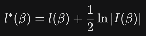
where,
l(β) : the standard log-likelihood for logistic regression
|l(β)| : the determinant of the Fisher information matrix

While standard logistic regression works best with perfect data, Firth’s stays stable even when your data is messy or limited.

In my previous post, I demonstrated how to calculate probabilities for standard logistic regression by hand. However, Firth’s Logistic Regression involves complex penalized likelihood functions that make manual calculation practically impossible. Fortunately, R offers a straightforward way to implement this model.

R function: logistf()

Here is one dataset. Let’s say this data is about how different immune volume affect the survival of plants.

if(!require(readr)) install.packages("readr")
library(readr)

github="https://raw.githubusercontent.com/agronomy4future/raw_data_practice/refs/heads/main/dosage_volume.csv"
df=data.frame(read_csv(url(github),show_col_types = FALSE))
set.seed(100)

print(df[sample(nrow(df),5),])
    object dosage.volume survival
102    102             0        1
112    112             0        0
4        4             0        0
55      55            61        1
70      70             0        1
.
.
.

First, I’ll conduct logistic regression.

logistic=glm(survival~dosage.volume, family="binomial", data=df)
summary(logistic)

Warning message:
glm.fit: fitted probabilities numerically 0 or 1 occurred 

Call:
glm(formula = survival ~ dosage.volume, family = "binomial", 
    data = df)

Coefficients:
              Estimate Std. Error z value Pr(>|z|)    
(Intercept)    -1.2767     0.2389  -5.343 9.14e-08 ***
dosage.volume   1.4282     0.3710   3.850 0.000118 ***
---
Signif. codes:  0 ‘***’ 0.001 ‘**’ 0.01 ‘*’ 0.05 ‘.’ 0.1 ‘ ’ 1

(Dispersion parameter for binomial family taken to be 1)

    Null deviance: 206.64  on 149  degrees of freedom
Residual deviance: 119.78  on 148  degrees of freedom
AIC: 123.78

Number of Fisher Scoring iterations: 10

The warning “glm.fit: fitted probabilities numerically 0 or 1 occurred” is the computer’s way of saying: “I found a pattern that is too perfect, and it is breaking my math.” Imagine you are testing a new drug. If every single person in the treatment group recovered, and no one in the control group recovered, you have what we call “Perfect Separation.”

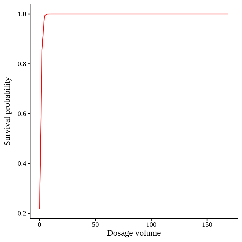
(exp(1.4282)-1) * 100 # 317.1184

It means when dosage volume unit increase 1, the odds of survival increases 317 times, which means dosage is extremely strong treatment. Let’s create a graph.

if(!require(ggplot2)) install.packages("ggplot2")
library(ggplot2)

ggplot(df, aes(x=dosage.volume, y=survival)) + 
  stat_smooth(method="glm", method.args=list(family="binomial"), se=FALSE, color="red", linewidth=0.7, formula='y~x') +
  labs(x="Dosage volume", y="Survival probability") +
  theme_classic(base_size=18, base_family="serif")+
  theme(legend.position="none",
        legend.title=element_blank(),
        axis.line=element_line(linewidth=0.5, colour="black"))

OutterProb= data.frame(Outter = seq(min(df1_na$Outter, na.rm=TRUE), 
                                  max(df1_na$Outter, na.rm=TRUE), 
                                  length.out = 100))
OutterProb$px= predict(logistic, newdata= OutterProb, type= "response")

summary= data.frame(Outter = c(0, 1, 2, 3, 4, 5, 170))
summary$prob= predict(logistic, newdata=summary, type="response")

print(summary)
  Outter      prob
1      0 0.2005514
2      1 0.5241399
3      2 0.8286544
4      3 0.9550240
5      4 0.9893879
6      5 0.9975631
7    170 1.0000000

When dosage volume become 5 out of 170, all plants are survived. This is so extreme case. To avoid this case, we can use logistf() function.

■ R function: logistf()

if(!require(logistf)) install.packages("logistf")
library(logistf)

and let’s run the code.

if(!require(logistf)) install.packages("logistf")
library(logistf)

logistic2= logistf(survival ~ dosage.volume, data= df)
summary(logistic2)

logistf(formula = survival ~ dosage.volume, data = df, plcontrol = logistpl.control(maxit = 10000))

Model fitted by Penalized ML
Coefficients:
                    coef   se(coef) lower 0.95 upper 0.95    Chisq            p
(Intercept)   -0.8781408 0.19619395 -9.8139503  -1.223453 12.72652 3.605076e-04
dosage.volume  0.3000209 0.05573791  0.1800398   4.319741 55.33396 1.016964e-13
              method
(Intercept)        2
dosage.volume      2

Method: 1-Wald, 2-Profile penalized log-likelihood, 3-None

Likelihood ratio test=55.33444 on 1 df, p=1.016964e-13, n=150
Wald test = 36.28995 on 1 df, p = 1.700388e-09

Now, the output is changed.

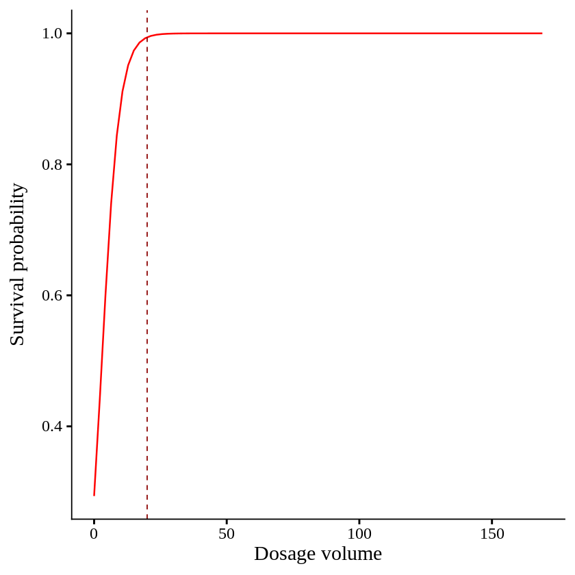
(exp(0.3000209)-1) * 100   # 34.989

When dosage volume unit increase 1, the odds of survival increases 34.989 times.

dosageProb= data.frame(dosage.volume = seq(min(df$dosage.volume, na.rm=TRUE), 
                                  max(df$dosage.volume, na.rm=TRUE), 
                                  length.out = 100))
dosageProb$px= predict(logistic2, newdata= dosage.volumeProb, type= "response")

summary= data.frame(dosage.volume = c(0,5,10,15,20,170))
summary$prob= predict(logistic2, newdata=summary, type="response")

print(summary)
  dosage.volume      prob
1             0 0.2935632
2             5 0.6506650
3            10 0.8930297
4            15 0.9739711
5            20 0.9940729
6           170 1.0000000

When dosage volume become 20 out of 170, all plants are survived.

ggplot() +
  geom_line(data = dosage.volumeProb, aes(x = dosage.volume, y = px), 
            color = "grey25", linewidth = 0.5) +
    
  geom_vline(xintercept=20, linetype= "dashed", color="darkred", linewidth=0.5) +  
    
  scale_x_continuous(breaks = seq(0, 150, 30), limits = c(0, 150)) +
  scale_y_continuous(breaks = seq(0, 1, 1), limits = c(0, 1)) +
  labs(x = "Number of tillers (>20cm radius)", 
       y = "Non-survival to Non-survival") +
  theme_classic(base_size = 18, base_family = "serif") +
  theme(legend.position = "none",
        axis.line = element_line(linewidth = 0.5, colour = "black"))

---