When analyzing grain size, we’ve used high-throughput image scanning machines. However, if we can detect grains using R code, estimating grain size becomes possible. In my previous R function, colorcapture(), we were able to detect fruit size and estimate its surface area in 2D.

[R package] Segment and Measure Colored Objects in Images (Feat. colorcapture)

Recently, I developed a new R function called phenokio() specifically designed to estimate the grain area of cereals.

1. Install the function

Before installing, please download Rtools (https://cran.r-project.org/bin/windows/Rtools)

if(!require(remotes)) install.packages("remotes")
if (!requireNamespace("phenokio", quietly = TRUE)) {
    remotes::install_github("agronomy4future/phenokio", force= TRUE)
}
library(remotes)
library(phenokio)

2. Default Values Summary Table

If a parameter is not explicitly defined in the phenokio() function, the following default values from the source code will be applied

Parameter	Default Value	Description
image_real_cm	c(20, 20)	Real-world area captured in the image (20cm x 20cm).
lower_hsv	c(0, 0, 0)	Minimum HSV bound (starts from pure black).
upper_hsv	c(180, 255, 255)	Maximum HSV bound (includes all colors).
extra_hsv	NULL	No secondary color masking is applied.
margin	0	No exclusion zone at the image borders.
k_open	c(5, 5)	Kernel size for noise removal.
open_iter	1	Number of times the noise removal is repeated.
k_close	c(7, 7)	Kernel size for closing gaps/cracks.
close_iter	2	Number of times the gap-filling is repeated.
fill_holes	FALSE	Does not automatically fill internal voids.
min_component_area_px	200	Ignores objects smaller than 200 pixels.
object_min_area_cm2	0.01	Ignores objects smaller than $0.01 cm^2$.
rel_min_frac_of_largest	0.00	Relative size filtering is disabled.
max_keep	2000	Limits the output to the 2,000 largest objects.
outline_color	“green”	Detection boundaries are rendered in green.
outline_thickness	2	Boundary line thickness set to 2 pixels.
ignore_processed_images	TRUE	Skips files that have already been analyzed.

3. Each code explainedFile & Path Settings

3.1. File & Path Settings

phenokio(
# --- File & Path Settings ---
input_folder="C:/Users/Coding",  #Directory path for source images
output_folder="C:/Users/Coding/output", #Directory path for saving processed results
image_real_cm=c(20, 20), #Physical dimensions of the captured area (Width, Height in cm)

First, you need to set the file paths for where the original images are saved (input_folder), as well as where the processed images will be saved (output_folder). Additionally, specify the actual size of the image frame (e.g., 20, 20). These values will vary depending on the height at which the image was taken.

3.2. Primary Color Segmentation (HSV)

# Target: Yellowish seed coat tones
lower_hsv=c(10, 80, 70),  #Lower bound for Hue, Saturation, and Value
upper_hsv=c(35, 255, 255), #Upper bound for Hue, Saturation, and Value
# --- Secondary Color Segmentation (extra_hsv) ---
# Target: Darker hilum (seed eye) or deep brown textures
extra_hsv=list(
   list(lower=c(0, 0, 10), upper=c(180, 255, 100)) 
   ),

This is an example for soybean grains. If the grain colors vary, for instance, due to the hilum in soybeans, you can add extra_hsv= to provide additional color segmentation.

There are many websites where you can visually check Hue (H), Saturation (S), and Value (V), allowing you to configure the HSV values to match your specific grain colors.

https://www.rapidtables.com/web/color/html-color-codes.html

3.3. Pre-processing & Noise Reduction

margin=10,   #Exclude pixels within 10px of the image border to avoid edge noise
k_open=c(3, 3),  #Kernel size for "Opening" (removes small background noise/dust)
open_iter= 1,    #Number of iterations for the opening operation
k_close=c(5, 5), #Kernel size for "Closing" (bridges small gaps/cracks within seeds)
close_iter=2,    #Number of iterations for the closing operation
fill_holes=TRUE, #Force-fill internal voids (useful for high-contrast spots on seeds)

You can set up noise threshold. Here is a concise explanation of each parameter used in the phenokio function:

margin = 10
This setting creates a 10-pixel "dead zone" around the very edge of your image. Any pixels or objects touching this border are ignored.
* Higher value: Safer against edge noise, but you lose more usable area for seeds.
* Lower value: Maximizes analysis area but may catch "ghost" objects at the image boundaries.
#
k_open = c(3, 3) & open_iter = 1
Opening is a cleaning process that performs "erosion" followed by "dilation." It effectively deletes objects smaller than the 3 x 3 kernel (like dust or tiny debris) while preserving the size of the actual seeds.
* Higher values: More aggressive cleaning of background noise; however, it may "shave off" the sharp tips of pointed seeds (like rice or awns).
* Lower values: Keeps the seed shape more authentic but might leave "pepper" noise in the background.
#
3. k_close = c(5, 5) & close_iter = 2
Closing is the opposite of opening; it performs "dilation" followed by "erosion." It acts like a bridge, connecting small gaps or cracks within a single seed that might be caused by shadows or surface texture.
* Higher values: Stronger at joining fragmented parts of a seed, but carries a high risk of "fusing" two seeds that are sitting close together into one giant object.
* Lower values: Better at separating individual seeds but might cause a single cracked seed to be counted as two separate pieces.
#
4. fill_holes = TRUE
This is crucial for seeds with high-contrast spots (like the hilum of a soybean) or shiny reflections that the color filter might otherwise think are "holes" in the middle of the grain.
* TRUE: Ensures the total area calculation includes the entire seed surface, even if the center is a different color.
* FALSE: The area calculation will subtract any "holes" or spots found inside the seed, likely leading to an underestimated size.

3.4. Filtering & Selection Criteria

min_component_area_px=50,  #Absolute minimum pixel count to be considered a candidate
object_min_area_cm2=0.03,   #Minimum physical area (cm2) to filter out non-seed debris
rel_min_frac_of_largest=0.1,  #Relative filter: ignore objects smaller than 10% of the largest detected seed
max_keep=500,  #Maximum number of objects to detect per image

You can configure the Filtering & Selection Criteria below. Here is a concise explanation of each parameter used in the phenokio function:

min_component_area_px = 50
This is the first-stage filter based on the raw digital image. It tells the software to ignore any group of pixels smaller than 50 total pixels. 
* Higher value: Speeds up processing by ignoring more "junk," but might delete very small or shriveled seeds.
* Lower value: Captures every tiny detail, but increases the risk of processing non-seed artifacts.
#
object_min_area_cm2 = 0.03
After the software converts pixels to centimeters, it checks if the object is at least 0.03cm2. This is highly effective for filtering out non-seed debris (like broken husk pieces or small stones) that might be the same color as your seeds but are physically too small to be a grain.
* Higher value: Useful when your sample has a lot of small trash or broken seed fragments you want to ignore.
* Lower value: Necessary if you are analyzing naturally tiny seeds like Arabidopsis or rapeseed.
#
rel_min_frac_of_largest = 0.1
At 0.1, it automatically ignores anything smaller than 10% of the largest seed's size. 
* Higher value (e.g., 0.5): Very strict; it will only keep objects that are at least half the size of the biggest seed.
* Lower value (e.g., 0.01): Very permissive; allows a wide range of seed sizes to be recorded in the same image.
#
max_keep = 500
It tells the function to stop recording after it finds the 500 best candidates (sorted by size).
* Higher value: Necessary for high-density images where you might have 1,000+ grains spread out (like rice or wheat).
* Lower value: Useful for keeping the data clean when you know you only placed a specific, small number of seeds (e.g., 50 soybeans) on the tray.

3.5. Visualization Style

  outline_color="green",        #Color of the detection boundary (contour)
  outline_thickness=7           #Thickness of the contour line in pixels
)

Finally, you can customize the visualization styles for how the processed grain images are displayed.

■ Code example for soybean

phenokio(
  input_folder="C:/Users/Coding",  
  output_folder="C:/Users/Coding/output", 
    image_real_cm=c(20, 20), 
    lower_hsv=c(10, 80, 70),  
    upper_hsv=c(35, 255, 255), 
    extra_hsv=list(
      list(lower=c(0, 0, 10), upper=c(180, 255, 100))),
    margin=10,   
    k_open=c(3, 3),  
    open_iter= 1,    
    k_close=c(5, 5),
    close_iter=2,   
    fill_holes=TRUE, 
    min_component_area_px=50,  
    object_min_area_cm2=0.03, 
    rel_min_frac_of_largest=0.1,  
    max_keep=500,                
    outline_color="green",       
    outline_thickness=5        
)

■ Code example for black bean

phenokio(
  input_folder="C:/Users/Coding",  
  output_folder="C:/Users/Coding/output", 
    image_real_cm=c(20, 20), 
    lower_hsv=c(0, 0, 0), 
    upper_hsv=c(180, 255, 60),
    extra_hsv=list(
      list(lower=c(0, 0, 10), upper=c(180, 255, 100))),
    margin=20,          
    k_open=c(3, 3),     
    open_iter=1,
    k_close=c(11, 11),      
    close_iter=2,
    fill_holes=TRUE,     
    min_component_area_px= 300, 
    object_min_area_cm2=0.1,
    rel_min_frac_of_largest=0.1, 
    max_keep=500, 
    outline_color="orange",  
    outline_thickness=5
  )

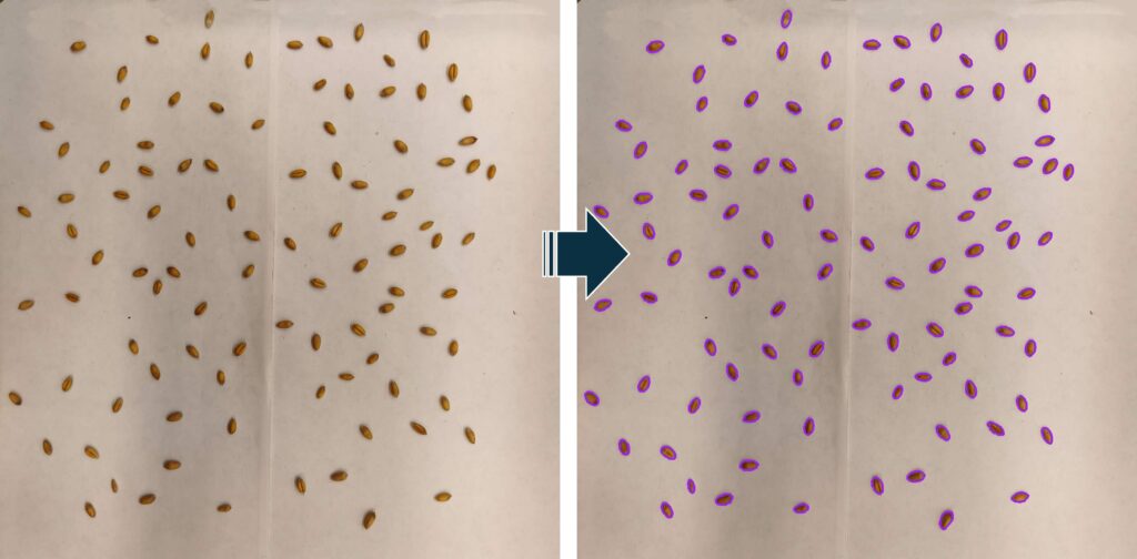
■ Code example for wheat

phenokio(
  input_folder="C:/Users/Coding",  
  output_folder="C:/Users/Coding/output", 
    image_real_cm=c(20, 20), 
    lower_hsv=c(0, 80, 50), 
    upper_hsv=c(179, 255, 255),
    extra_hsv=list(
      list(lower=c(0, 0, 10), upper=c(180, 255, 100))),
    margin=10,          
    k_open=c(3, 3),     
    open_iter=1,
    k_close=c(5, 5),      
    close_iter=1,
    fill_holes=TRUE,     
    min_component_area_px=100, 
    object_min_area_cm2=0.01,
    rel_min_frac_of_largest=0.1, 
    max_keep=500, 
    outline_color="purple",  
    outline_thickness=4
)

■ Utilizing Grain Morphometric Data

Unlike average grain weight, which typically provides only a single data point per treatment, the area data generated by phenokio() allows for distribution analysis. Instead of a simple bar graph, you can use normal distribution curves (histograms) to determine the ‘source’ of a yield decrease: Is the entire grain population smaller, or has the proportion of shriveled, smaller grains simply increased?

---