In this session, I will introduce the method of calculating the Best Linear Unbiased Estimator (BLUE). Instead of simply listing formulas as many websites do to explain BLUE, this post aims to help readers understand the process of calculating BLUE with an actual dataset using R.
I have the following data.
df= structure(list(location = c("Cordoba", "Cordoba", "Cordoba", "Cordoba", "Cordoba", "Cordoba", "Cordoba", "Cordoba", "Cordoba", "Cordoba", "Cordoba", "Cordoba", "Granada", "Granada", "Granada", "Granada", "Granada", "Granada", "Granada", "Granada", "Granada", "Granada", "Granada", "Granada", "Granada", "Granada", "Granada", "Granada", "Leon", "Leon", "Leon", "Leon", "Leon", "Leon", "Leon", "Leon", "Leon", "Leon", "Leon", "Leon"), trt = c(0L, 24L, 36L, 48L, 0L, 24L, 36L, 48L, 0L, 24L, 36L, 48L, 0L, 24L, 36L, 48L, 0L, 24L, 36L, 48L, 0L, 24L, 36L, 48L, 0L, 24L, 36L, 48L, 0L, 24L, 36L, 48L, 0L, 24L, 36L, 48L, 0L, 24L, 36L, 48L), block = structure(c(2L, 2L, 2L, 2L, 3L, 3L, 3L, 3L, 4L, 4L, 4L, 4L, 1L, 1L, 1L, 1L, 2L, 2L, 2L, 2L, 3L, 3L, 3L, 3L, 4L, 4L, 4L, 4L, 1L, 1L, 1L, 1L, 3L, 3L, 3L, 3L, 4L, 4L, 4L, 4L), levels = c("1", "2", "3", "4"), class = "factor"), yield = c(780, 1280, 1520, 1130, 790, 1300, 1525, 1140, 800, 10, 15, 11, 10, 1490, 1790, 1345, 1066, 1510, 1700, 1355, 948, 1560, 1830, 1368, 960, 1550, 1866, 1356, 800, 1250, 1550, 910, 663.6, 1260, 1480, 900, 750, 1195, 1525, 900)), row.names = c(NA, -40L), class = "data.frame")
The dataset comprises three different locations involving four sulfur experiments organized into four blocks for crop yield; however, some blocks were missing in Cordoba and Leon.
df$block= as.factor(df$block)
print(df)

   location trt block  yield
1   Cordoba   0     2  780.0
2   Cordoba  24     2 1280.0
3   Cordoba  36     2 1520.0
4   Cordoba  48     2 1130.0
5   Cordoba   0     3  790.0
6   Cordoba  24     3 1300.0
7   Cordoba  36     3 1525.0
8   Cordoba  48     3 1140.0
9   Cordoba   0     4  800.0
10  Cordoba  24     4   10.0
11  Cordoba  36     4   15.0
12  Cordoba  48     4   11.0
13  Granada   0     1   10.0
14  Granada  24     1 1490.0
15  Granada  36     1 1790.0
16  Granada  48     1 1345.0
17  Granada   0     2 1066.0
18  Granada  24     2 1510.0
19  Granada  36     2 1700.0
20  Granada  48     2 1355.0
21  Granada   0     3  948.0
22  Granada  24     3 1560.0
23  Granada  36     3 1830.0
24  Granada  48     3 1368.0
25  Granada   0     4  960.0
26  Granada  24     4 1550.0
27  Granada  36     4 1866.0
28  Granada  48     4 1356.0
29     Leon   0     1  800.0
30     Leon  24     1 1250.0
31     Leon  36     1 1550.0
32     Leon  48     1  910.0
33     Leon   0     3  663.6
34     Leon  24     3 1260.0
35     Leon  36     3 1480.0
36     Leon  48     3  900.0
37     Leon   0     4  750.0
38     Leon  24     4 1195.0
39     Leon  36     4 1525.0
40     Leon  48     4  900.0
Block 1 is missing from the Cordoba data, and Block 2 is missing from Leon. Do you think it is acceptable to use this unbalanced data as is, or should we apply a method to compensate for the imbalance?
To help you understand, let’s use a very simple analogy.

Three Students taking a 4-Set Exam. Imagine three students  are taking an exam. The exam consists of four different sets.

Student A: Completed both the easy Set 1 and the difficult Set 2 (Average Score: 50)
Student B: Completed only the difficult Set 2 (Average Score: 30)

If we only look at the simple average, Student A (50) seems smarter than Student B (30). We might wrongly conclude that Student B is a poor student.

The BLUE (Mixed Model) Approach
The Mixed Model doesn't just look at the final score; it looks at the context (i.e., Random effect).

The model analyzes all the data and realizes, "Wait, everyone scored 20 points lower on Set 2 because it was much harder." Since Student B only tackled the most difficult set, the model adjusts the score: "If Student B had also taken the easy set, they likely would have scored a 50 as well." The model concludes that the actual ability (Fixed Effect) of Student A and Student B is actually similar.

# Fixed Effect: The actual underlying factor we want to measure (e.g., student ability or crop yield).
# Random/Block Effect: The environmental noise or context that can bias the results (e.g., difficulty of the exam set or soil quality of a specific block).
# Adjusted Means: The "fair" scores calculated after removing the bias of the blocks.
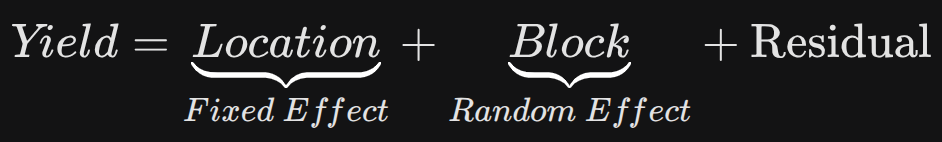
Consider a dataset investigating crop yields in three regions of Spain under sulfur fertilizer treatments. The experiment was conducted using four repetitions as blocks. In this model, location is defined as a fixed factor, while block are defined as random factors (For now, let’s disregard sulfur, assuming its effect is consistent across all locations.).
In such a mixed-effects model, the Best Linear Unbiased Estimator (BLUE) is used to estimate the fixed effects, while the Best Linear Unbiased Prediction (BLUP) is used to predict the random effects. I will now demonstrate how to calculate both the BLUEs and BLUPs using R.

To calculate BLUE using R
I will configure the model. Location is set as a fixed factor, while block are set as a random factor. The model configuration is as follows.
if(!require(lme4)) install.packages("lme4")
if(!require(lmerTest)) install.packages("lmerTest")
library(lme4)
library(lmerTest)

model=lmer(yield ~ 0 +   location + (1|block), data=df)
The reason I set up the intercept as 0 is because I want the model to directly estimate the mean yield (BLUE) for each specific location, rather than calculating the differences relative to a reference region.
Why suppressing the Intercept?
When configuring the model asyield ~ 0 + location + (1|block), we are using what is known as a "Cell-Means Model." This setup is chosen for the following reasons:
1. Direct Estimation of Absolute Means (BLUEs)
In a default model (yield ~ location), R treats the first alphabetical location as a reference level (intercept) and shows other locations as differences from that baseline. By adding 0 (or -1), we remove this baseline. This forces the model to calculate the absolute mean yield for every location directly. These resulting coefficients are the BLUEs (Best Linear Unbiased Estimators) for each specific region.
2. Efficiency in Reporting and Interpretation
If the primary goal of your study is to report the actual productivity of each of the three Spanish regions, the 0 + location approach is much more efficient. You can extract the results using fixef(model) and report them immediately without having to manually add the intercept to the slope coefficients.
3. Objective Comparison Without Bias
Treating one specific region as a "standard" (intercept) can sometimes lead to biased interpretations in comparative studies. Suppressing the intercept ensures that each region is treated as an independent fixed factor, providing a more balanced and objective view of the geographic yield distribution.
4. Handling Unbalanced Data through BLUE
As we discussed, when data is unbalanced (e.g., some blocks are missing in certain regions), the 0 + location setup ensures that the estimate for each region is adjusted for the random effects of the blocks. The model looks at the block performance across other regions to "correct" the missing or skewed data in a specific region, providing the most "unbiased" version of that region's mean.
In summary: You use 0 + location because you want the model outputs to represent the true, adjusted average yield (BLUE) of each location, rather than just showing how much they differ from a reference point.
Let’s see the output of the model.
summary(model)

Linear mixed model fit by REML. t-tests use Satterthwaite's method [
lmerModLmerTest]
Formula: yield ~ 0 + location + (1 | block)
   Data: df

REML criterion at convergence: 565.8

Scaled residuals:
    Min      1Q  Median      3Q     Max
-2.9351 -0.6253  0.1773  0.6523  1.3901

Random effects:
 Groups   Name        Variance Std.Dev.
 block    (Intercept)  15481   124.4
 Residual             199021   446.1
Number of obs: 40, groups:  block, 4

Fixed effects:
                Estimate Std. Error      df t value Pr(>|t|)
locationCordoba   846.05     145.85   11.73   5.801 9.27e-05 ***
locationGranada  1356.50     127.71    9.25  10.622 1.73e-06 ***
locationLeon     1123.10     145.85   11.73   7.701 6.38e-06 ***
---
Signif. codes:  0 ‘***’ 0.001 ‘**’ 0.01 ‘*’ 0.05 ‘.’ 0.1 ‘ ’ 1

Correlation of Fixed Effects:
            lctnCr lctnGr
locatinGrnd 0.208
locationLen 0.167  0.208
In the lmer output, the three values listed under the Estimate column in the Fixed effects section (846.05, 1356.50, 1123.10) are indeed the BLUE (Best Linear Unbiased Estimator) values for each location.
Why are these values called "BLUE"?

□ Best and Unbiased: These are not just simple arithmetic means of the collected data. They are the most "unbiased" optimal estimates, obtained by statistically adjusting (removing) the noise from random effects (Block) included in the model.

□ Location-Specific: Because you used the 0 + location syntax, these values represent the pure adjusted mean for each specific region, rather than the difference relative to a reference baseline.
# Fixed Effects: Population-level average regression coefficients (Named Vector)
print(data.frame(fixef(model)))

                fixef.model.
locationCordoba     846.0555
locationGranada    1356.5000
locationLeon       1123.0997
Let’s see the arithmetic mean of each location.
if(!require(dplyr)) install.packages("dplyr")
library(dplyr)

structure = df %>%
       group_by(location) %>%
       dplyr::summarize(
       across(
        .cols= yield,
        .fns= list(
         Mean= ~mean(., na.rm= TRUE),
         n= ~length(.),
         se= ~sd(., na.rm= TRUE) / sqrt(length(.)))),
        .groups= "drop") %>%
        as.data.frame()

print(structure)
  location yield_Mean yield_n  yield_se
1  Cordoba   858.4167      12 164.48544
2  Granada  1356.5000      16 114.23204
3     Leon  1098.6333      12  91.43936
You can see the arithmetic (simple) mean is different from BLUE.
| Location | Simple mean | BLUE |
| Cordoba | 858.4167 | 846.05 |
| Granada | 1356.5000 | 1356.50 |
| Leon | 1098.6333 | 1123.10 |
While the simple mean only averages the available observed data, BLUE provides a more balanced estimate by accounting for both missing blocks and localized yield anomalies. For Cordoba, the model identifies that the exceptionally low yields in Block 4 are a ‘block-specific’ issue rather than a regional one, and it also leverages data from other regions to compensate for the poor/missing information in Block 1.
In the case of Leon, which lacks any data for Block 2, the model uses the performance of Block 2 in Granada and Cordoba to estimate what Leon’s yield would have been. Since Block 2 generally shows higher yields, BLUE adjusts Leon’s estimate upward to reflect its true potential. By ‘filling in’ these gaps and adjusting for the noise in Cordoba’s Block 4, BLUE offers a far more accurate representation of each region’s productivity than the biased simple mean.
For Granada, where the experimental design was perfectly balanced across all blocks and treatments, the simple mean and the BLUE are identical. This confirms that there was no regional bias or missing information to be adjusted in Granada, unlike Cordoba and Leon, where BLUE corrected for missing blocks and localized yield anomalies
Now let’s calculate the prediction values from the model and add these prediction values into the existing data.
df$prediction= predict (model, re.form = NA)
Now let’s calculate the average of these prediction values.
if(!require(dplyr)) install.packages("dplyr")
library(dplyr)

summary = df %>%
       group_by(location) %>%
       dplyr::summarize(
       across(
        .cols= prediction,
        .fns= list(
         Mean= ~mean(., na.rm= TRUE),
         n= ~length(.),
         se= ~sd(., na.rm= TRUE) / sqrt(length(.)))),
        .groups= "drop") %>%
        as.data.frame()
print(summary)
  location prediction_Mean prediction_n prediction_se
1  Cordoba        846.0555           12             0
2  Granada       1356.5000           16             0
3     Leon       1123.0997           12             0
Did you find that the mean of prediction values from the model is the same as BLUE and also standard error becomes 0?
print(df)
   location trt block  yield prediction
1   Cordoba   0     2  780.0   846.0555
2   Cordoba  24     2 1280.0   846.0555
3   Cordoba  36     2 1520.0   846.0555
4   Cordoba  48     2 1130.0   846.0555
5   Cordoba   0     3  790.0   846.0555
6   Cordoba  24     3 1300.0   846.0555
7   Cordoba  36     3 1525.0   846.0555
8   Cordoba  48     3 1140.0   846.0555
9   Cordoba   0     4  800.0   846.0555
10  Cordoba  24     4   10.0   846.0555
11  Cordoba  36     4   15.0   846.0555
12  Cordoba  48     4   11.0   846.0555
13  Granada   0     1   10.0  1356.5000
14  Granada  24     1 1490.0  1356.5000
15  Granada  36     1 1790.0  1356.5000
16  Granada  48     1 1345.0  1356.5000
17  Granada   0     2 1066.0  1356.5000
18  Granada  24     2 1510.0  1356.5000
19  Granada  36     2 1700.0  1356.5000
20  Granada  48     2 1355.0  1356.5000
21  Granada   0     3  948.0  1356.5000
22  Granada  24     3 1560.0  1356.5000
23  Granada  36     3 1830.0  1356.5000
24  Granada  48     3 1368.0  1356.5000
25  Granada   0     4  960.0  1356.5000
26  Granada  24     4 1550.0  1356.5000
27  Granada  36     4 1866.0  1356.5000
28  Granada  48     4 1356.0  1356.5000
29     Leon   0     1  800.0  1123.0997
30     Leon  24     1 1250.0  1123.0997
31     Leon  36     1 1550.0  1123.0997
32     Leon  48     1  910.0  1123.0997
33     Leon   0     3  663.6  1123.0997
34     Leon  24     3 1260.0  1123.0997
35     Leon  36     3 1480.0  1123.0997
36     Leon  48     3  900.0  1123.0997
37     Leon   0     4  750.0  1123.0997
38     Leon  24     4 1195.0  1123.0997
39     Leon  36     4 1525.0  1123.0997
40     Leon  48     4  900.0  1123.0997
Using predict(model, re.form = NA) means ŷ = Fixed Effect (Location). It ignores which block the data came from. It asks: “What is the general potential of this location if we strip away the luck of having a good or bad block? All values at each location will get the exact same value. The standard error of these values is 0 because you are looking at a single constant estimate (the BLUE).
On the other hand, using predict(model) means ŷ = Fixed Effect (Location) + Random Effect (Block). It accounts for the specific conditions of that data point. It asks: “Based on what we know about this specific block and this specific treatment, what was the most likely yield?” If you include random factors using df$prediction2 = predict(model), it means you are calculating the ‘Subject-level’ (or group-level) prediction. This value represents the expected yield for a specific observation by combining the regional average (BLUE) with the specific deviations of the block (BLUPs) associated with that row.
# Random Effects: Group-specific deviations/offsets from the population average (List of Dataframes)
print(data.frame(ranef(model)))

  grpvar        term grp   condval   condsd
1  block (Intercept)   1 -37.08357 97.68736
2  block (Intercept)   2  73.39903 97.68736
3  block (Intercept)   3  58.81900 89.48238
4  block (Intercept)   4 -95.13446 89.48238
Look at the prediction2 values in the data below. prediction2 represents ŷ = Fixed Effect (Location) + Random Effect (Block). If I subtract the condval (Conditional Value) of each block from prediction2, the resulting value is the population-level prediction (Fixed Effect only). For example, 919.4545 – 73.39903 ≈ 846.055.
df$prediction2=predict (model)
print(df)

   location trt block  yield prediction prediction2
1   Cordoba   0     2  780.0   846.0555    919.4545
2   Cordoba  24     2 1280.0   846.0555    919.4545
3   Cordoba  36     2 1520.0   846.0555    919.4545
4   Cordoba  48     2 1130.0   846.0555    919.4545
5   Cordoba   0     3  790.0   846.0555    904.8745
6   Cordoba  24     3 1300.0   846.0555    904.8745
7   Cordoba  36     3 1525.0   846.0555    904.8745
8   Cordoba  48     3 1140.0   846.0555    904.8745
9   Cordoba   0     4  800.0   846.0555    750.9210
10  Cordoba  24     4   10.0   846.0555    750.9210
11  Cordoba  36     4   15.0   846.0555    750.9210
12  Cordoba  48     4   11.0   846.0555    750.9210
13  Granada   0     1   10.0  1356.5000   1319.4164
14  Granada  24     1 1490.0  1356.5000   1319.4164
15  Granada  36     1 1790.0  1356.5000   1319.4164
16  Granada  48     1 1345.0  1356.5000   1319.4164
17  Granada   0     2 1066.0  1356.5000   1429.8990
18  Granada  24     2 1510.0  1356.5000   1429.8990
19  Granada  36     2 1700.0  1356.5000   1429.8990
20  Granada  48     2 1355.0  1356.5000   1429.8990
21  Granada   0     3  948.0  1356.5000   1415.3190
22  Granada  24     3 1560.0  1356.5000   1415.3190
23  Granada  36     3 1830.0  1356.5000   1415.3190
24  Granada  48     3 1368.0  1356.5000   1415.3190
25  Granada   0     4  960.0  1356.5000   1261.3655
26  Granada  24     4 1550.0  1356.5000   1261.3655
27  Granada  36     4 1866.0  1356.5000   1261.3655
28  Granada  48     4 1356.0  1356.5000   1261.3655
29     Leon   0     1  800.0  1123.0997   1086.0161
30     Leon  24     1 1250.0  1123.0997   1086.0161
31     Leon  36     1 1550.0  1123.0997   1086.0161
32     Leon  48     1  910.0  1123.0997   1086.0161
33     Leon   0     3  663.6  1123.0997   1181.9187
34     Leon  24     3 1260.0  1123.0997   1181.9187
35     Leon  36     3 1480.0  1123.0997   1181.9187
36     Leon  48     3  900.0  1123.0997   1181.9187
37     Leon   0     4  750.0  1123.0997   1027.9652
38     Leon  24     4 1195.0  1123.0997   1027.9652
39     Leon  36     4 1525.0  1123.0997   1027.9652
40     Leon  48     4  900.0  1123.0997   1027.9652
In the Cordoba region, Block 4 exhibited exceptionally low observed yields (10.0–15.0). However, the linear mixed-effects model adjusted these values; when calculating conditional predictions; predict(model), the estimate for Block 4 rose to 750.92. This adjustment occurs because the model accounts for the overall block-level variance through Best Linear Unbiased Predictors (BLUPs). Notably, the mean of these conditional predictions remains mathematically identical to the simple arithmetic mean of the observed data because the BLUPs are centered around the group mean to minimize residuals.
summary = df %>%
       group_by(location) %>%
       dplyr::summarize(
       across(
        .cols= c(prediction, prediction2),
        .fns= list(
         Mean= ~mean(., na.rm= TRUE),
         n= ~length(.),
         se= ~sd(., na.rm= TRUE) / sqrt(length(.)))),
        .groups= "drop") %>%
        as.data.frame()

summary= subset(summary,
         select=c(location,prediction_Mean,prediction_se,
         prediction2_Mean,prediction2_se))

print(summary)
  location prediction_Mean prediction_se prediction2_Mean prediction2_se
1  Cordoba        846.0555             0         858.4167       22.98831
2  Granada       1356.5000             0        1356.5000       17.92245
3     Leon       1123.0997             0        1098.6333       19.14033
To report the Best Linear Unbiased Estimators (BLUEs)—the true adjusted means—one must instead utilize the fixed-effects estimates by excluding random factors adding re.form = NA. The standard error for these BLUEs represents the uncertainty of the fixed-effect estimate and should be obtained from the model’s fixed-effects covariance matrix or via specialized packages like emmeans, rather than calculating the standard deviation of the predicted constants.
How to calculate standard error of BLUE?
The standard error (SE) of the Best Linear Unbiased Estimators (BLUEs) was calculated using the emmeans() package for the following reasons
First, unlike simple arithmetic means, emmeans()
Second, while the standard deviation of raw predictions often fails to reflect model uncertainty, emmeans() derives the SE directly from the fixed-effects covariance matrix.
Finally, the package utilizes the Kenward-Roger degrees-of-freedom approximation, which is the gold standard for providing robust SEs and confidence intervals in linear mixed-effects models, ensuring that the precision of each regional estimate is accurately represented regardless of sample size differences.
if(!require(emmeans)) install.packages("emmeans")
library(emmeans)

model= lmer(yield ~ 0 + location + (1|block), data = df)
output= emmeans(model, "location")
print(output)

 location emmean  SE    df lower.CL upper.CL
 Cordoba     846 151 11.30      515     1177
 Granada    1356 128  8.88     1067     1646
 Leon       1123 151 11.30      792     1455

Degrees-of-freedom method: kenward-roger
Confidence level used: 0.95
We aim to develop open-source code for agronomy ([email protected])
© 2022 – 2025 https://agronomy4future.com – All Rights Reserved.
Last Updated: 04/07/2026