The Gamma distribution is a flexible family of continuous probability distributions defined only for non-negative values (x>0). It’s commonly used to model quantities that represent time, size, or waiting periods—anything that can’t go below zero and often shows right-skewed behavior (a long tail toward larger values).

In essence, the Gamma distribution describes how likely different positive values are to occur, determined by two key parameters: the shape (α) and the scale (θ). Together, these parameters control the curve’s form and spread, allowing the Gamma distribution to model a broad range of real-world processes.

---

Why Use the Gamma Distribution?

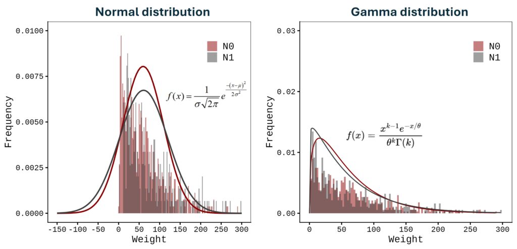
The Gamma distribution is often preferred over the Normal distribution for modeling strictly positive and asymmetric data. For instance, if you model grain weight with a Normal distribution and the variability is high relative to the mean, the left tail of the bell curve will extend into negative values—an impossible outcome. The Gamma model naturally avoids this issue because its support starts at zero.

Moreover, the Gamma distribution can capture a wide variety of shapes—from highly skewed to nearly symmetrical—making it ideal for describing random processes such as rainfall amounts, lifetimes of devices, or waiting times in queuing systems.

---

■ Parameters and their Effects

1. Shape Parameter (α)

■ Role: Determines the overall shape and the number of modes (peaks).
■ Effect:
□ When α<1, the distribution is L-shaped, with the highest density near zero.

□ When α=1, the Gamma distribution simplifies to the Exponential distribution, often used for modeling waiting times between independent events.

□ As α increases, the distribution becomes more symmetric and bell-shaped, gradually approaching the Normal distribution as a limiting case.

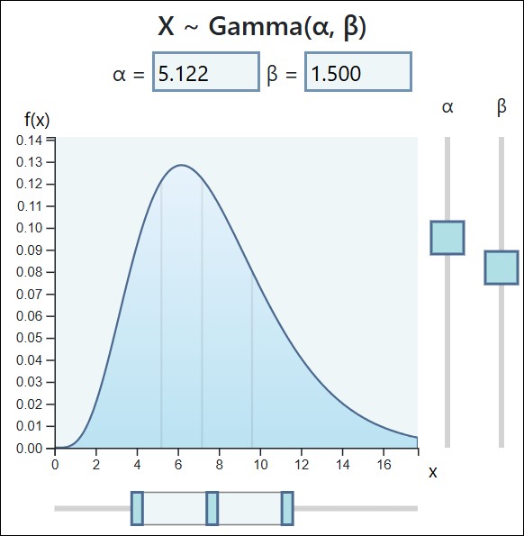
2. Scale Parameter (θ)

■ Role: Stretches or compresses the distribution along the x-axis.
■ Effect:
□ A larger θ value spreads the distribution out (increasing variance), while a smaller θ value makes it more concentrated around the mean.

□ The mean of the Gamma distribution is E[X]=αθ , and the variance is Var(X)=αθ2
→ I’ll explain about this using the actual dataset.

How to calculate Shape, Scale and Probability Density Function (PDF)

The equation for the probability density function (PDF) of the Gamma Distribution can be found on Wikipedia.

Most people, I believe, stop at this point in their effort to understand the Gamma Distribution’s PDF; however, grasping the underlying principle reduces the concept to a middle-school math level.

First, let’s calculate the shape parameter. Here is some example data for practice.

df= data.frame(No= c(1:30), 
               Weight= c(99.5, 8.7, 51, 46.3, 71.4, 81.4, 56.3, 61.4, 24.4, 14.7, 83.4, 
                         6.1, 4.9, 180.7, 134.8, 133.5, 90.6, 38, 37.8, 17.1, 97.4, 4.8, 
                         54.5, 89.1, 123.9, 25.3, 74.3, 64.3, 226.7, 2.9))

head(df,5)
  No. Weight
1   1   99.5
2   2    8.7
3   3   51.0
4   4   46.3
5   5   71.4
.
.
.

The Maximum Likelihood Estimation (MLE) Equation

To find the MLE for the shape parameter α, you must solve a specific equation that equates the theoretical properties of the Gamma distribution to the characteristics of your observed data. The equation is:

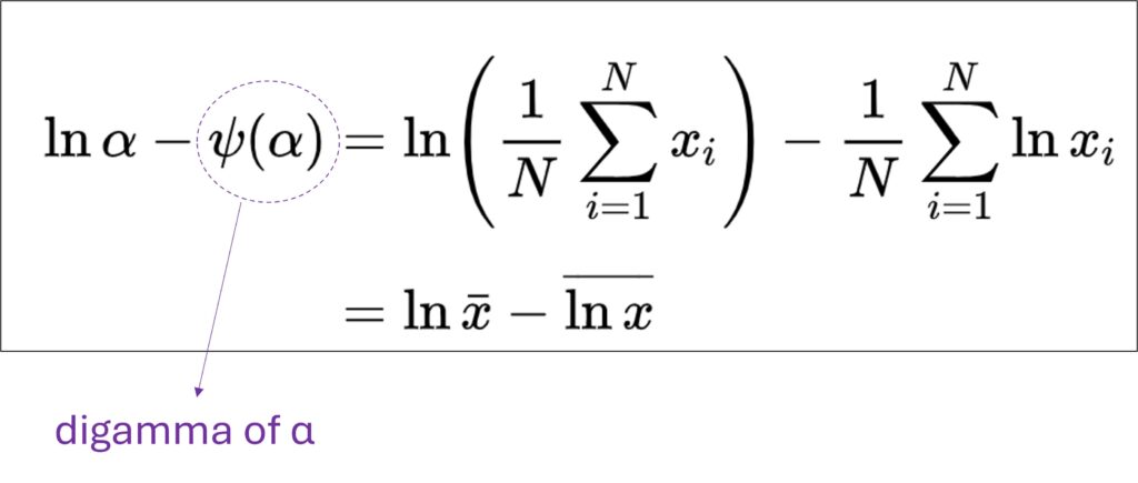
where:
α is the maximum likelihood estimate for the shape parameter.
ψ(α) is the Digamma function evaluated at the estimated shape parameter.
ln(α) is the natural logarithm of the estimated shape parameter.
x̄ is the mean of the observed data.
ln(x) bar is the mean of the natural logarithms of the observed data.

Let’s go through the calculation step by step.

head(df,5)
  No. Weight
1   1   99.5
2   2    8.7
3   3   51.0
4   4   46.3
5   5   71.4
.
.
.

No.	Weight
1	99.5
2	8.7
3	51.0
4	46.3
5	71.4
.	.
30	2.9

First, the mean weight is calculated as 66.84; thus, x̄ = 66.84.

No.	Weight	Weight_mean (x̄)
1	99.5	66.84
2	8.7
3	51.0
4	46.3
5	71.4
.	.
30	2.9

Second, the natural logarithm of the mean, ln(66.84), is 4.20.

No.	Weight	Weight_mean (x̄)	ln(x̄)
1	99.5	66.84	4.20 = ln(66.84)
2	8.7
3	51.0
4	46.3
5	71.4
.	.
30	2.9

Third, let’s calculate ln(x).

No.	Weight	Weight_mean (x̄)	ln(x̄)	ln(x)
1	99.5	66.84	4.20 = ln(66.84)	4.60 = ln(99.5)
2	8.7			2.16
3	51.0			3.93
4	46.3			3.84
5	71.4			4.27
.	.			.
30	2.9			1.06 = ln(2.9)
			Mean	3.74

and also calculate the mean of ln(x).

No.	Weight	Weight_mean (x̄)	ln(x̄)	ln(x)	Mean of ln(x)
1	99.5	66.84	4.20 = ln(66.84)	4.60 = ln(99.5)	3.74
2	8.7			2.16
3	51.0			3.93
4	46.3			3.84
5	71.4			4.27
.	.			.
30	2.9			1.06 = ln(2.9)

According to the equation below, let’s calculate the difference between ln(x̄) and the mean of ln(x). The result is 0.46 ( = 4.20 – 3.74).

Therefore, ln(α) – ψ(α) = 0.46.

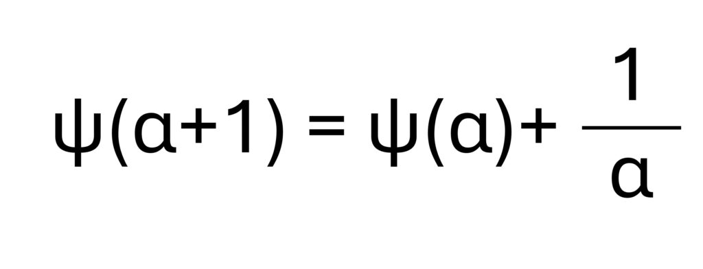
In the digamma function of α, ψ(1) = −γ = −0.5772, where γ is the Euler–Mascheroni constant. The following equation is then suggested.

α	ln(α)	ψ(α)	ln(α) – ψ(α)
1.0	0.0000	−0.5772	−0.5772
1.2	0.1823	ψ(1.25) ≈ ψ(1) +0.2*[ψ(2)−ψ(1)] ≈ -0.5772 + 0.2*(0.4228+0.5772) ≈ – 0.3772	0.4055 – (-0.3772) =0.7827
1.5	0.4055	ψ(1.25) ≈ ψ(1) +0.5*[ψ(2)−ψ(1)] ≈ -0.5772 + 0.5*(0.4228+0.5772) ≈ – 0.0772	0.4055 – (- 0.0772) = 0.4827
2.0	0.6931	0.4228 ≈ −0.5772 + 1/1	0.2703

In the Digamma function ψ(α), we know that ψ(1)=−γ=−0.5772, where γ is the Euler–Mascheroni constant. Based on this relationship, the following equation is often used to estimate the shape parameter α of the gamma distribution. From this observations, I estimate that the shape parameter α is approximately 1.5. However, it is not possible to calculate the exact value of α manually, since the gamma distribution is nonlinear and involves special functions that typically require numerical methods or iterative estimation (such as maximum likelihood estimation). Here, I have only outlined the basic concept behind the calculation process of α.

Scale (θ) is calculated as x̄ / α. Therefore, when α = 1.5, θ = 44.56 ( = 66.84 / 1.5 ).

gammacurve() R package

I recently developed an R package, gammacurve(), which simplifies the calculation of the shape (α) and scale (θ) parameters, as well as the PDF and CDF.

First, install the package as follows.

if(!require(remotes)) install.packages("remotes")
if (!requireNamespace("gammacurve", quietly = TRUE)) {
  remotes::install_github("agronomy4future/gammacurve", force= TRUE)
}
library(remotes)
library(gammacurve)

and run gammacurve() as shown below.

df= data.frame(No= c(1:30), 
               Weight= c(99.5, 8.7, 51, 46.3, 71.4, 81.4, 56.3, 61.4, 24.4, 14.7, 83.4, 
                         6.1, 4.9, 180.7, 134.8, 133.5, 90.6, 38, 37.8, 17.1, 97.4, 4.8, 
                         54.5, 89.1, 123.9, 25.3, 74.3, 64.3, 226.7, 2.9))

outputPDF= gammacurve(df, variable="Weight", func=1)
print(head(outputPDF,3))
  Weight    No alpha_hat theta_hat PDF
1    0      NA      1.23      54.4 0      
2    2.9    30      1.23      54.4 0.00977
3    4.8    22      1.23      54.4 0.0106 
.
.
.

The gammacurve() function automatically provides the shape (α) and scale (θ) parameters. The shape (α) is 1.23. My manual calculation was close, but not entirely accurate. As mentioned earlier, manual calculation cannot yield a fully precise shape (α) because the curve is not linear.

When the shape (α) is 1.23, the scale (θ) is calculated as x̄ / α. Given that the mean weight is 66.84, the scale (θ) is 66.84 / 1.23 ≈ 54.4, which matches the value provided by gammacurve().

Now that we know both the shape (α) and scale (θ), we can calculate the probability density function (PDF) curve using Excel.

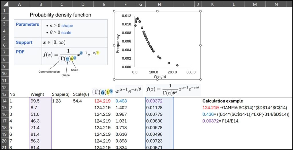
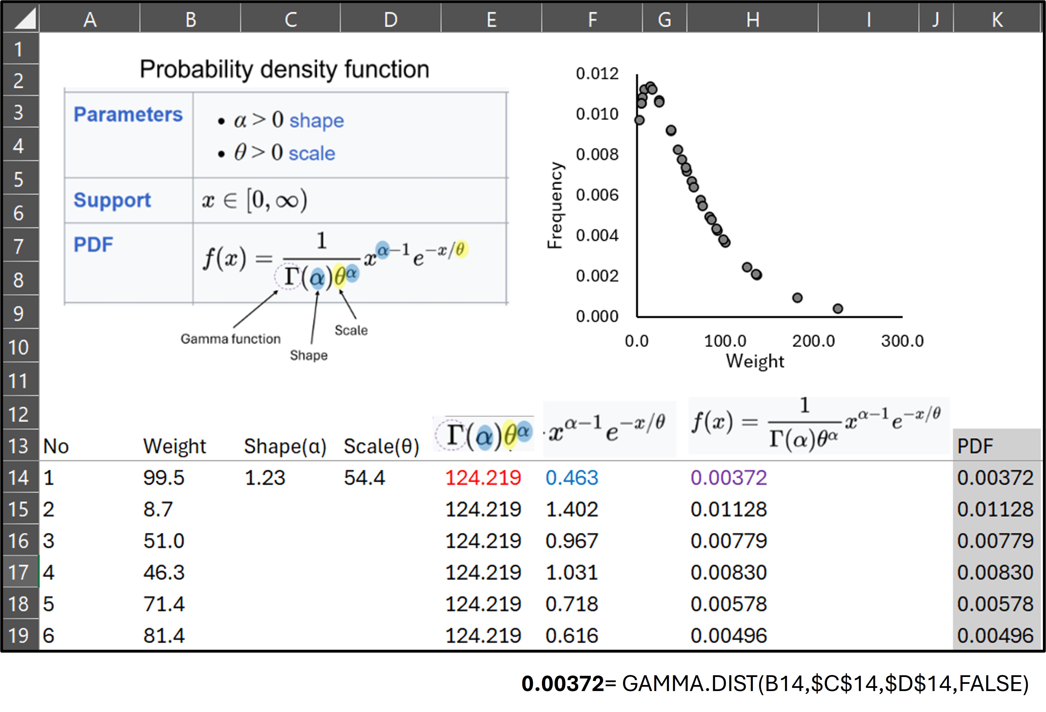
I calculated the probability density function (PDF), but you don’t need to do it manually—Excel provides the GAMMA.DIST() function.

GAMMA.DIST(X, α, θ , FALSE) #FALSE: PDF / TRUE: CDF

and If you use GAMMA.DIST(), you can obtain the PDF, and it is exactly the same as what I calculated manually.

Now, let’s return to the gammacurve() function.”

outputPDF= gammacurve(df, variable="weight", func=1)
print(head(outputPDF,3))
  Weight    No alpha_hat theta_hat PDF
1    0      NA      1.23      54.4 0      
2    2.9    30      1.23      54.4 0.00977
3    4.8    22      1.23      54.4 0.0106 
.
.
.

I’ll downlod the outputPDF data.

if(!require(writexl)) install.packages("writexl")
library(writexl)
write_xlsx (outputPDF,"C:/Users/agron/Desktop/outputPDF.xlsx")
# Please check the pathway in your computer

Then, compare the PDF values with those calculated in Excel. They are the same.

A slight difference can be observed between the two results, which arises from variations in numerical precision. When the data table is output as a data frame, the precise shape (α) value is 1.229772.

outputPDF= gammacurve(df, variable="Weight", func=1)
outputPDF=data.frame(outputPDF)

print(head(outputPDF,3))
  Weight No alpha_hat theta_hat         PDF
1    0.0 NA  1.229772  54.35152 0.000000000
2    2.9 30  1.229772  54.35152 0.009766344
3    4.8 22  1.229772  54.35152 0.010588496 
.
.
.

In Excel, the shape parameter (α) was set to 1.23, resulting in a negligible difference. Nonetheless, the outcomes are practically identical, confirming that gammacurve() accurately calculates the Probability Density Function (PDF).

Next, we will create the Gamma distribution.

gplot(data=outputPDF, aes(x=Weight)) +   
  geom_line(data=outputPDF, aes(x=Weight, y=PDF), color="darkred") +
  #scale_x_continuous(breaks=seq(-150,300,50), limits=c(-150,300)) +
  scale_y_continuous(breaks=seq(0,0.02,0.005), limits=c(0,0.02)) +
  labs(x="Weight", y="Frequency") +
  theme_classic(base_size=15, base_family="serif") +
  theme(legend.position="none",
        panel.border= element_rect(color="black", fill=NA, linewidth=0.5),
        axis.line=element_line(linewidth=0.5, colour="black"))

gammacurve(): An Efficient R Package for Gamma Distribution

If you’ve followed this post, you now understand how the probability density function (PDF) for the Gamma distribution is derived and can calculate it by hand and in Excel. Simply using an Excel function or R code won’t fully convey the underlying principles, which is why I explained the steps. If you now fully understand the Gamma distribution, you can use the gammacurve() package to easily obtain the PDF and the cumulative distribution function (CDF).

Now, let’s use another dataset.

if(!require(remotes)) install.packages("readr")
library (readr)

github="https://raw.githubusercontent.com/agronomy4future/raw_data_practice/refs/heads/main/sweet_potato_weight.csv"
df=data.frame(read_csv(url(github),show_col_types = FALSE))

print(head(df,3))
       Season Nitrogen Block   weight
1 2020_Season       N1     I 111.8380
2 2020_Season       N1     I   9.7788
3 2020_Season       N1     I  57.3240

This dataset represents fruit weight in response to different nitrogen levels across two seasons. First, let’s create a normal distribution graph. Due to variation in the data, the distribution curve includes negative values, which are not realistic—weight cannot be negative.

Fig1= ggplot(data=df, aes(x=weight, fill=Nitrogen)) +
  stat_function(data=subset(df,Nitrogen=="N0"),aes(x=weight, color=Nitrogen),
                size=1,fun=dnorm, 
                args=c(mean=mean(subset(df, Nitrogen=="N0")$weight),
                       sd=sd(subset(df, Nitrogen=="N0")$weight))) +
  stat_function(data=subset(df,Nitrogen=="N1"),aes(x=weight, color=Nitrogen),
                size=1,fun=dnorm, 
                args=c(mean=mean(subset(df, Nitrogen=="N1")$weight),
                       sd=sd(subset(df, Nitrogen=="N1")$weight))) +
  scale_fill_manual(values=c("darkred","grey25"))+
  scale_color_manual(values= c("darkred", "grey25")) +
  scale_x_continuous(breaks=seq(-150,300,50), limits=c(-150,300)) +
  scale_y_continuous(breaks=seq(0,0.01,0.005), limits=c(0,0.01)) +
  facet_wrap(~ Season) +
  labs(x="Fruit weight", y="Frequency") +
  theme_classic(base_size=15, base_family="serif") +
  theme(legend.position=c(0.85, 0.85),
        legend.title=element_blank(),
        legend.key=element_rect(color="white", fill="white"),
        legend.text=element_text(family="serif", face="plain", size=15, color= "Black"),
        legend.background=element_rect(fill="white"),
        strip.background=element_rect(color="white", linewidth=0.5, linetype="solid"),
        strip.text = element_text(size = 18),
        panel.border= element_rect(color="black", fill=NA, linewidth=0.5),
        axis.line=element_line(linewidth=0.5, colour="black"))

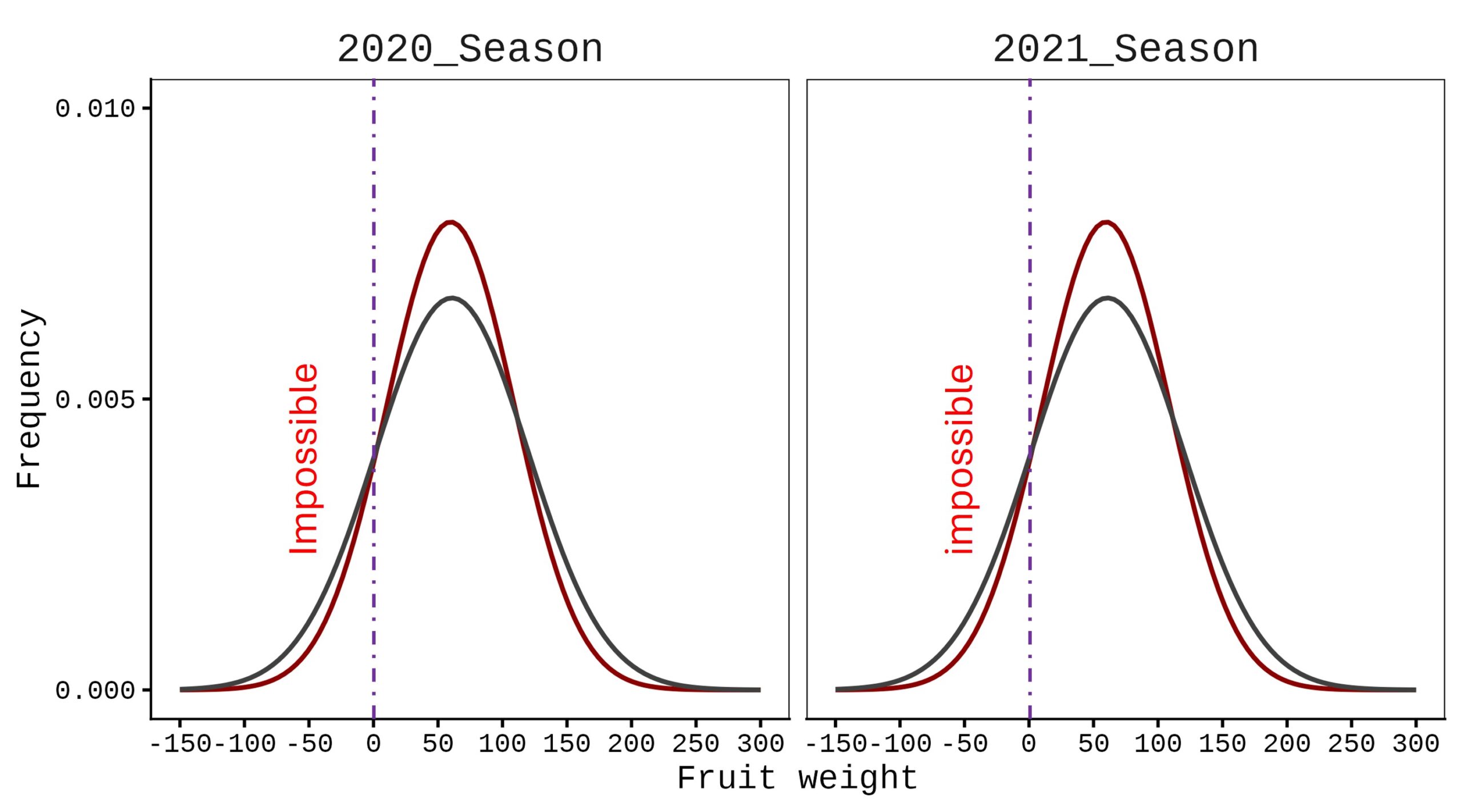
In this case, a normal distribution is not appropriate; instead, a Gamma distribution should be applied.

if(!require(remotes)) install.packages("remotes")
if (!requireNamespace("gammacurve", quietly = TRUE)) {
  remotes::install_github("agronomy4future/gammacurve", force= TRUE)
}
library(remotes)
library(gammacurve)

output= gammacurve(df, variable="weight", group=c("Season","Nitrogen"), func=1)

print(head(output,3))
 Season        Nitrogen  weight  Block  alpha_hat  theta_hat  PDF
1 2020_Season  N0        0       NA          1.33       41.4  0      
2 2020_Season  N0        2.14    IV          1.33       41.4  0.00956
3 2020_Season  N0        2.47    IV          1.33       41.4  0.00996
.
.
.

ggplot(data=output, aes(x=weight, fill=Nitrogen)) +
  geom_histogram(aes(y=0.5*..density..), alpha=0.5,
                 position='identity', binwidth=2.5) +
  geom_line(data=output, aes(x=weight, y=PDF, group=Nitrogen, color=Nitrogen)) +
  scale_fill_manual(values=c("darkred","grey25"))+
  scale_color_manual(values= c("darkred", "grey25")) +
  scale_x_continuous(breaks=seq(0,300,50), limits=c(0,300)) +
  scale_y_continuous(breaks=seq(0,0.03,0.01), limits=c(0,0.03)) +
  facet_wrap(~ Season) +
  guides(color="none") +
  labs(x="Potato tuber weight (g)", y="Frequency") +
  theme_classic(base_size=15, base_family="serif") +
  theme(legend.position=c(0.85, 0.85),
        legend.title=element_blank(),
        legend.key=element_rect(color="white", fill="white"),
        legend.text=element_text(family="serif", face="plain", size=15, color= "Black"),
        legend.background=element_rect(fill="white"),
        strip.background=element_rect(color="white", linewidth=0.5, linetype="solid"),
        strip.text = element_text(size = 18),
        panel.border= element_rect(color="black", fill=NA, linewidth=0.5),
        axis.line=element_line(linewidth=0.5, colour="black"))

If you want to draw the cumulative distribution function (CDF), simply set func= 2.

output= gammacurve(df, variable="weight", group=c("Season","Nitrogen"), func=2)

print(head(output,3))
  Season       Nitrogen   weight  Block  alpha_hat  theta_hat    CDF
1 2020_Season  N0         0       NA          1.33       41.4      0     
2 2020_Season  N0         2.14    IV          1.33       41.4 0.0157
3 2020_Season  N0         2.47    IV          1.33       41.4 0.0189
.
.
.

ggplot(data=output, aes(x=weight, fill=Nitrogen)) +
  geom_line(data=output, aes(x=weight, y=CDF, group=Nitrogen, color=Nitrogen)) +
  scale_fill_manual(values=c("darkred","grey25"))+
  scale_color_manual(values= c("darkred", "grey25")) +
  scale_x_continuous(breaks=seq(0,300,50), limits=c(0,300)) +
  scale_y_continuous(breaks=seq(0,1,0.1), limits=c(0,1)) +
  facet_wrap(~ Season) +
  guides(color="none") +
  labs(x="Potato tuber weight (g)", y="Frequency") +
  theme_classic(base_size=15, base_family="serif") +
  theme(legend.position=c(0.88, 0.13),
        legend.title=element_blank(),
        legend.key=element_rect(color="white", fill="white"),
        legend.text=element_text(family="serif", face="plain", size=15, color= "Black"),
        legend.background=element_rect(fill="white"),
        strip.background=element_rect(color="white", linewidth=0.5, linetype="solid"),
        strip.text = element_text(size = 18),
        panel.border= element_rect(color="black", fill=NA, linewidth=0.5),
        axis.line=element_line(linewidth=0.5, colour="black"))

---

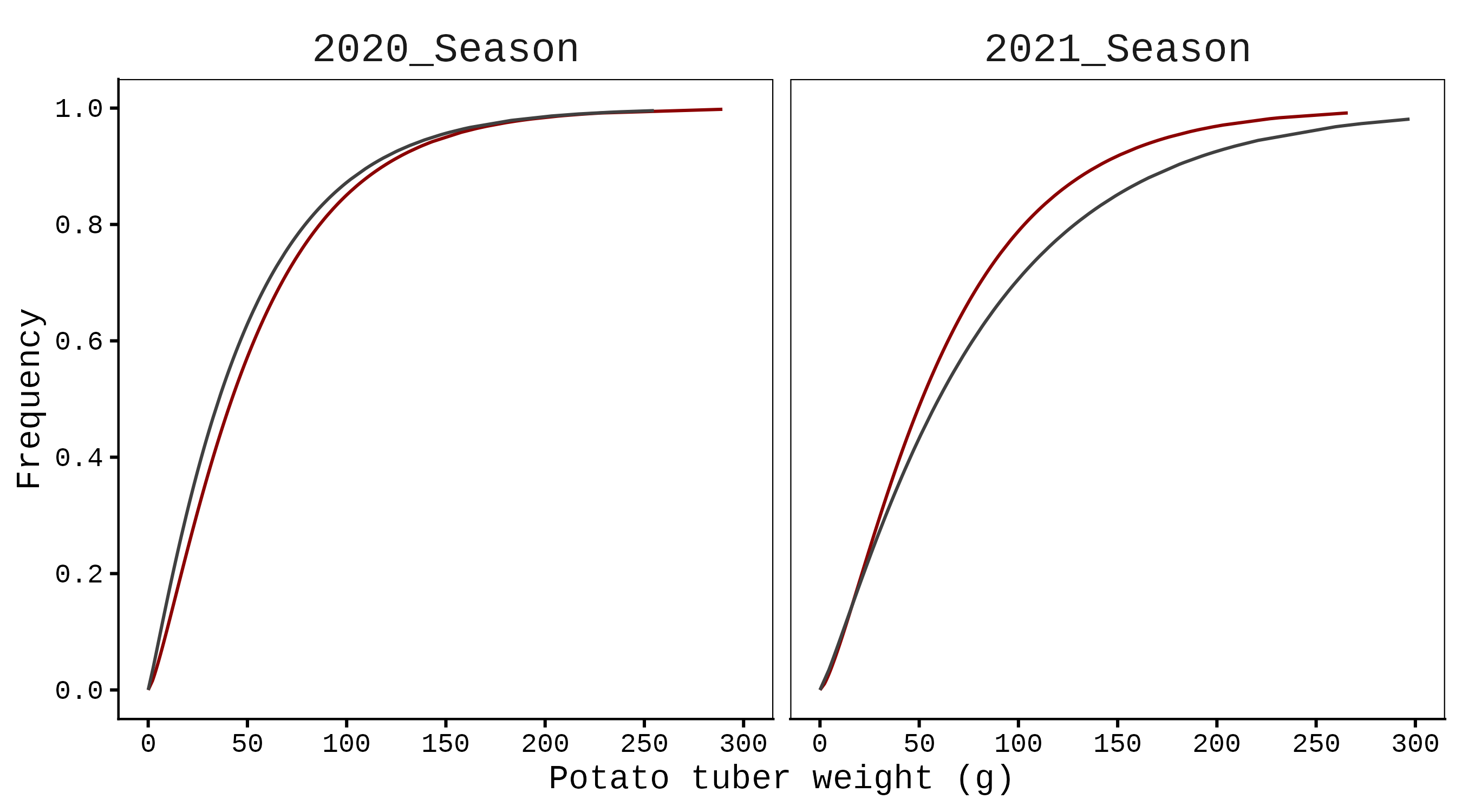
To draw the Gamma distribution curve, I used a line graph without any additional statistical processing, since gammacurve() already provides the probability density function (PDF) and cumulative distribution function (CDF).