---

Recently, I’ve been focusing on Bayesian statistics. To organize the concepts for myself as well, I’m going to explain Bayes’ theorem as simply as possible.

Let’s import a dataset from Kaggle.

https://www.kaggle.com/datasets/cameronseamons/electronic-sales-sep2023-sep2024

This dataset contains information used to analyze customer purchasing behavior at an electronics store. You can download it from Kaggle after creating an account.

I’ll load the data directly using Python code. I’m using Google Colab.

from google.colab import drive
import pandas as pd
import zipfile
import os

drive.mount('/content/drive')

! mkdir -p ~/.kaggle
! cp "/content/drive/MyDrive/0. Colab/2_Coding/Statistics/Database/kaggle.json" ~/.kaggle
! chmod 600 ~/.kaggle/kaggle.json

!kaggle datasets download -d cameronseamons/electronic-sales-sep2023-sep2024 -p "/content/drive/MyDrive/0. Colab/2_Coding/Statistics/Database"

sales= "/content/drive/MyDrive/0. Colab/2_Coding/Statistics/Database/electronic-sales-sep2023-sep2024.zip"

sales_path= "/content/drive/MyDrive/0. Colab/2_Coding/Statistics/Database"

with zipfile.ZipFile(sales, 'r') as zip_ref:
     zip_ref.extractall(sales_path)

%cd /content/drive/MyDrive/0. Colab/2_Coding/Statistics/Database

sales= pd.read_csv("Electronic_sales_Sep2023-Sep2024.csv", index_col=0)

print(sales.head(3))
             Age Gender Loyalty Member Product Type      SKU  Rating  \
Customer ID                                                            
1000          53   Male             No   Smartphone  SKU1004       2   
1000          53   Male             No       Tablet  SKU1002       3   
1002          41   Male             No       Laptop  SKU1005       3   

            Order Status Payment Method  Total Price  Unit Price  Quantity  \
Customer ID                                                                  
1000           Cancelled    Credit Card      5538.33      791.19         7   
1000           Completed         Paypal       741.09      247.03         3   
1002           Completed    Credit Card      1855.84      463.96         4   

            Purchase Date Shipping Type              Add-ons Purchased  \
Customer ID                                                              
1000           2024-03-20      Standard  Accessory,Accessory,Accessory   
1000           2024-04-20     Overnight                   Impulse Item   
1002           2023-10-17       Express                            NaN   

             Add-on Total  
Customer ID                
1000                40.21  
1000                26.09  
1002                 0.00  
.
.
.

This is how I imported the dataset directly from Kaggle. For more details, please refer to the post below.

How to import Kaggle datasets directly into Google Colab?

If you find this process too complicated, you can simply download the dataset from Kaggle and upload it to your own Google Drive.

There is information in this dataset such as gender, loyalty membership status, product type, and payment method. Using this data, let’s work through Bayes’ theorem step by step.

1. Probability

Probability represents “the likelihood of an event occurring out of all possible outcomes.” In our dataset, what is the probability that a randomly selected person is male? Let’s compute it directly using Python.

male= (sales['Gender']=="Male")
def prob(A):
    return (A.mean())

prob(male) 
# 0.5082

When we select a person from the dataset at random, the probability that the person is male, P(Male) is 50.82%. In simple terms, the dataset contains 20,000 rows in total, and 10,164 of those rows correspond to male customers. Therefore, the probability is simply 10,164 ÷ 20,000 = 0.5082.

male.sum() / len(sales)
# 0.5082

2. Logical conjunction

Next, let’s look at logical conjunction. A logical conjunction is simply another name for the AND operator. Given two statements, A and B, the conjunction “A AND B” is true only when both A and B are true; otherwise, it is false. In our dataset, we can use a logical conjunction to determine the probability that a randomly selected person is both male and purchased a tablet.

# the probability that a person is male
male= (sales['Gender']=="Male")
def prob(A):
    return (A.mean())

prob(male) 
# 0.5082

# the probability that a person purchases a tablet
tablet= (sales['Product Type']=="Tablet")
def prob(A):
  return A.mean()

prob(tablet)
# 0.2052

In other words, the probability of being male and purchasing a tablet; P(Male and Tablet) is 0.5082 × 0.2052 = 0.104. You can also compute this using the code below.

male= (sales['Gender']=="Male")
tablet= (sales['Product Type']=="Tablet")
def prob(A):
  return A.mean()

prob (male & tablet)
# 0.104

From the calculation above, we can see that a logical conjunction is commutative. In other words, A AND B is the same as B AND A. Therefore, the probability of “being male and purchasing a tablet”; P(Male and Tablet) is the same as the probability of “purchasing a tablet and being male P(Tablet and Male).

male= (sales['Gender']=="Male")
tablet= (sales['Product Type']=="Tablet")
def prob(A):
  return A.mean()

prob (tablet & male)
# 0.104

Here, I used the expression “and.” In fact, changing just this one word can completely change the probability calculation.

3. Conditional probability

Now, let’s move on to conditional probability. What I want to determine is the probability that a person purchased a tablet, given that the person is male; P(Tablet | Male).

Let’s calculate it in Python as follows.

tablet[male].sum() / male.sum() 
or
prob (tablet & male) / prob (male)
# 0.205

That probability is 20.5%. Do you see the difference?

The probability of being male and purchasing a tablet; P(Tablet and Male), was 10.4%. But the probability of purchasing a tablet given that the person is male; P(Tablet | Male), is 20.5%. A single change in wording leads to a completely different probability.

In the dataset, the total number of males was male.sum() = 10,164, and the number of males who purchased a tablet was tablet[male].sum() = 2,088. Therefore, the conditional probability is:

2,088 ÷ 10,164 = 0.205

This calculation can be expressed in code as follows.

def prob(A):
  return A.mean()

prob(tablet[male])
# 0.205

Let’s create a function called conditional to make the code a bit simpler.

def conditional (proposition, given):
  return prob(proposition[given])

conditional (tablet, male)
# 0.205

---

Here we encounter an important concept: “conditional probabilities are not commutative.”

In other words,

the probability of being male given that a person purchased a tablet”; P(Male | Tablet) is not the same as “the probability of purchasing a tablet given that a person is male; P(Tablet | Male).

In our dataset, the total number of tablet purchasers was tablet.sum() = 4,104, and among them, the number of males was male[tablet].sum() = 2,088.

So the conditional probability, P(Male | Tablet) is:

2,088 ÷ 4,104 = 0.509

male[tablet].sum() / tablet.sum()
# 0.509

def conditional (proposition, given):
  return prob(proposition[given])

conditional (male, tablet)
# 0.509

The probability of purchasing a tablet given that a person is male; P(Tablet | Male) is 20.5%, but the probability of being male given that a person purchased a tablet; P(Male | Tablet) is 50.9%. This shows that conditional probabilities are not interchangeable.

■ Basic probability laws

Earlier, we discussed probability, logical conjunction, and conditional probability. Now, let’s derive the relationships among these three concepts.

[1] Probability
P(A): The probability of event A.

[2] Logical Conjunction
P(A and B): The probability of the conjunction of A and B — that is, the probability that both A and B are true.

[3] Conditional Probability
P(A | B): The probability that A is true given that B has occurred.

Earlier, we found that the probability of purchasing a tablet given that the person is male is 0.205.

# P(A|B)
def conditional (proposition, given):
  return prob(proposition[given])

conditional (tablet, male)
# 0.205

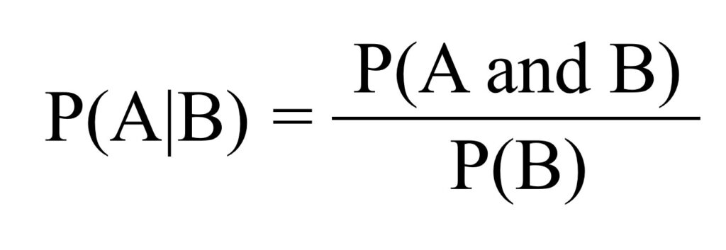
And we noted that this probability is calculated as follows.

# P(A and B) / P(B)
prob (tablet & male) / prob (male)
= 0.104 / 0.5082
# 0.205

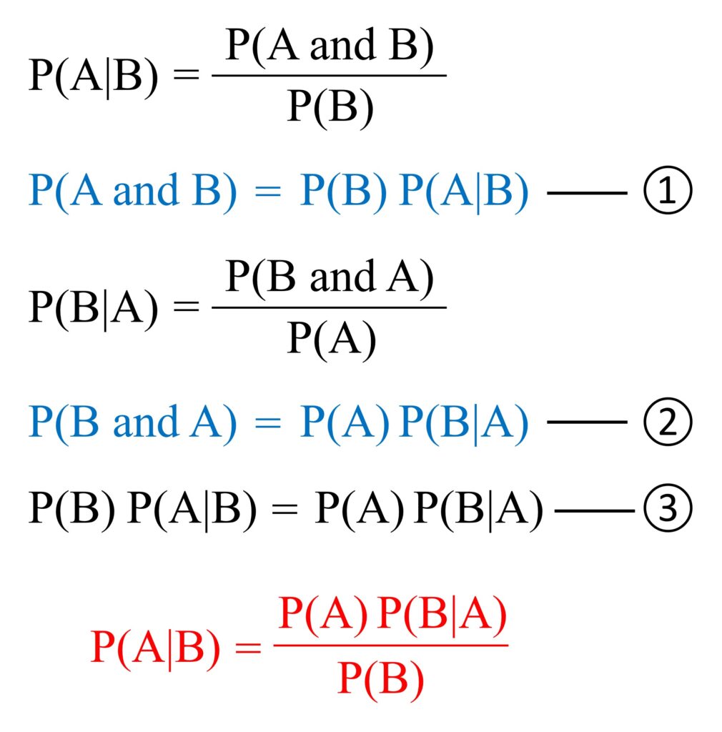
From this, we can derive the following formula.

This expression can be written as follows.

Then, we can also derive the following expression.

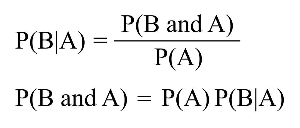
We stated earlier that logical conjunction is commutative; P(A and B) = P(B and A).
Therefore, the following expression holds.

The equation above can be rewritten as follows.

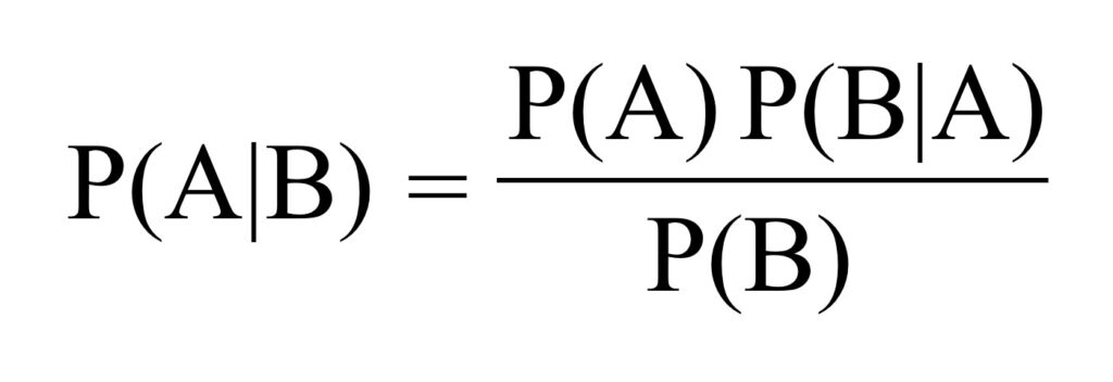
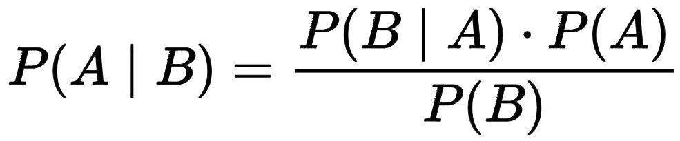
And this final expression is what we call Bayes’ theorem.

In other words, the probability of A given B is equal to the probability of A multiplied by the probability of B given A, divided by the probability of B.

■ Bayes’ theorem

---