□ Quantifying Phenotypic Plasticity of Crops
In my previous post, I explained how to quantify phenotypic plasticity in crops and described three different approaches: 1) Responsiveness, 2) Reaction Norm, and the 3) Finlay-Wilkinson Regression Model.
Responsiveness is calculated as (Treatment − Control) / Control. It indicates how the dependent variable (e.g., yield) responds to a given treatment relative to the control. The responsiveness value can range from −1 (complete reduction) to values greater than 0, depending on the magnitude of increase, and reflects plasticity. For more details, please refer to the post below.
□ [R package] Calculate the responsiveness of each treatment relative to a control (Feat. deltactrl)
The Finlay–Wilkinson Regression Model establishes a relationship between the environmental index and the dependent variable (e.g., yield), with the slope indicating the degree of plasticity of the genotype to environmental variation. For more details, please refer to the post below.
□ [R package] Finlay-Wilkinson Regression model (feat. fwrmodel)
Today, I’ll explain the last of the three concepts I suggested: the reaction norm, in detail.

What is reaction norm?
A reaction norm describes how the phenotype of a particular genotype changes across a range of environmental conditions. In simple terms, it’s the set of possible phenotypes that a single genotype can express when exposed to different environments.
The formula for a reaction norm depends on how you model the relationship between phenotype and environment for a given genotype. The most basic and widely used formulation — particularly in crop physiology — is a linear reaction norm model:
Pij= μ + Gi + βiEj + ϵij
Where:
Pij: Phenotypic value of genotype i in environment j
μ: Overall mean
Gi: Genotypic main effect (baseline performance of genotype i)
Ej: Environmental index or environmental variable (could be continuous or categorical)
βi: Genotype-specific sensitivity (slope of reaction norm; plasticity)
ϵij: Residual error
and this model could be simplified
P(E)= a + bE
Where:
P(E) = Phenotype as a function of environment E
a = Intercept (baseline phenotype)
b = Slope (sensitivity or plasticity of the phenotype to the environment)
E = Environmental variable
and the slope (b) is calculated as

Let’s calculate the slope manually. Let’s upload a dataset.
if(!require(readr)) install.packages("readr")
library(readr)
github="https://raw.githubusercontent.com/agronomy4future/raw_data_practice/refs/heads/main/fertilizer_treatment.csv"
df= data.frame(read_csv(url(github), show_col_types=FALSE))
set.seed(100)

print(df[sample(nrow(df),5),])
     Genotype Block    variable value
10 Genotype_C    II     Control  58.5
55 Genotype_B   III Fertilizer3  44.1
38 Genotype_B    II Fertilizer2  65.8
48 Genotype_D    IV Fertilizer2  51.0
51 Genotype_A   III Fertilizer3  28.3
.
.
.
Suppose this dataset contains crop yield data for different genotypes under different fertilizer applications.
data_overview= function(data) {
  cat_vars= data[, sapply(data, function(x) is.factor(x) || is.character(x))]
  cat_unique= lapply(cat_vars, unique)
    num_vars= names(data)[sapply(data, is.numeric)]
    cat("Categorical Variables (unique values):\n")
  print(cat_unique)
    cat("\nNumeric Variables (column names only):\n")
  print(num_vars)
}

data_overview(df)

Categorical Variables (unique values):
$Genotype
[1] "Genotype_A" "Genotype_B" "Genotype_C" "Genotype_D"

$Block
[1] "I"   "II"  "III" "IV"

$variable
[1] "Control"     "Fertilizer1" "Fertilizer2" "Fertilizer3"


Numeric Variables (column names only):
[1] "value"
There are 4 genotypes and 4 different fertilizer treatments, each with 4 replicates. My interest is in how the phenotype (crop yield) of each genotype changes across a range of environmental conditions (fertilizer levels). To investigate this, I’ll calculate the reaction norm for each genotype. First, let’s focus on Genotype_C
if(!require(dplyr)) install.packages("dplyr")
library(dplyr)

df1= data.frame(subset(df, Genotype=="Genotype_C") %>%
                    group_by(variable) %>%
                    dplyr::summarize(across(c(value),
                                            .fns= list(Mean=~mean(., na.rm= TRUE)))))
print(df1)
variable      value_Mean
Control       53.925
Fertilizer1   51.375
Fertilizer2   55.875
Fertilizer3   56.050
Step 1) Calculate Σ (Ej – Ē)2
In the explanation of the reaction norm model, I mentioned that the environmental variable can be either continuous or categorical. This means that even if we label treatments as “Control,” “Fertilizer 1,” and so on, these categories often correspond to actual quantitative values, such as 0 N kg/ha or 100 N kg/ha. While it is possible to use categorical values (e.g., 1, 2, 3) to represent treatments, using continuous values is generally preferable for quantifying the reaction norm, as it allows for a more precise characterization of the response across the environmental gradient.
Environment Ej | Phenotypic value (yield)Pi | (Ej – Ē) | (Ej – Ē)2 |
| Control = 0 | 53.925 | -100 (= 0 – 100) | 10000 |
| Fertilizer 1 = 50 | 51.375 | 50 | 2500 |
| Fertilizer 2 = 150 | 55.875 | 50 | 2500 |
| Fertilizer 3 = 200 | 56.050 | 100 | 10000 |
Ē= 100 | p̄i = 54.3 | Σ (Ej – Ē)2 =25000 |
Step 2) Calculate (Pij – P̅i)
Environment Ej | Phenotypic value (yield)Pi | (Ej – Ē) | (Ej – Ē)2 | (Pij – P̅i) |
| Control = 0 | 53.925 | -100 (= 0 – 100) | 10000 | -0.38 |
| Fertilizer 1 = 50 | 51.375 | 50 | 2500 | -2.93 |
| Fertilizer 2 = 150 | 55.875 | 50 | 2500 | 1.57 |
| Fertilizer 3 = 200 | 56.050 | 100 | 10000 | 1.74 |
Ē= 100 | p̄i = 54.3 | Σ (Ej – Ē)2 =25000 |
Step 3) Calculate Σ (Ej – Ē) (Pij – P̅i)
Environment Ej | Phenotypic value (yield)Pi | (Ej – Ē) | (Ej – Ē)2 | (Pij – P̅i) | Σ (Ej – Ē) (Pij – P̅i) |
| Control = 0 | 53.925 | -100 (= 0 – 100) | 10000 | -0.38 | 38.13 |
| Fertilizer 1 = 50 | 51.375 | -50 | 2500 | -2.93 | 146.56 |
| Fertilizer 2 = 150 | 55.875 | 50 | 2500 | 1.57 | 78.44 |
| Fertilizer 3 = 200 | 56.050 | 100 | 10000 | 1.74 | 174.37 |
Ē= 100 | p̄i = 54.3 | Σ (Ej – Ē)2 =25000 | Σ (Ej – Ē) (Pij – P̅i) = 437.50 |
Step 4) Calculate the slope
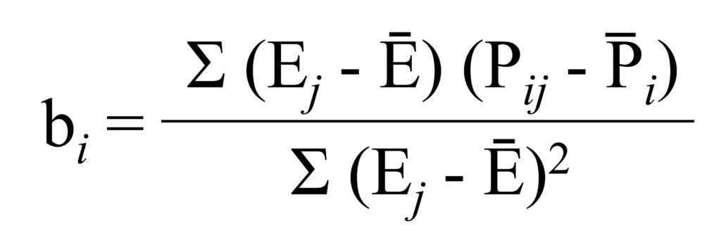
We can calculate the slope. It’s 437.50 / 25000 = 0.0175
Step 5) Calculate intercept
According to the model, P(E)= a + bE, we can calculate the intercept.
a = P(E) – bE, and P(E) is regarded as the grand mean of the yield, which is 54.3, and E is regarded as the grand mean of the environments which is 100, and we already calculated the slope as 0.0175. Therefore, a = 54.3 – 0.0175*100 = 52.55
Step 6) Final reaction norm equation:
Therefore, P(E) =52.55 + 0.0175*E
The genotype_C produces 52.55 Mg/ha at zero nitrogen, and for each additional 1 kg nitrogen, yield increases by 0.0175 Mg/ha (or (or 17.5 kg/ha).
At 0N (Control), the yield was 53.925, but the model says it’s 52.55 at 0N. The difference between 53.925 (observed) and 52.55 (estimated) is due to natural variation and the fact that the regression line minimizes overall squared error, not error at any single point.
This is the reaction norm: it tells you the linear response of yield to nitrogen for this genotype.
Genotypic plasticity in response to N fertilizer
This is the summary of the reaction norm model for each genotype.
| Genotype | Intercept | Slope | Reaction Norm Model |
| Genotype A | 42.91 | -0.0046 | P(E) = 42.91 – 0.0046*E |
| Genotype B | 52.48 | 0.0092 | P(E) = 52.48 + 0.0092*E |
| Genotype C | 52.56 | 0.0175 | P(E) = 52.55 + 0.0175*E |
| Genotype D | 62.49 | -0.0142 | P(E) = 62.49 – 0.0142*E |
Genotypes A and D show yield decreases as nitrogen increases (negative plasticity), while Genotypes B and C show yield increases with increasing nitrogen (positive plasticity).
Let’s calculate responsiveness. If I calculate responsiveness, it would be as shown below. I’ll use deltactrl() package I recently developed.
if(!require(remotes)) install.packages("remotes")
if (!requireNamespace("deltactrl", quietly = TRUE)) {
remotes::install_github("agronomy4future/deltactrl", force= TRUE)
}
library(remotes)
library(deltactrl)

df1= deltactrl(
  data= df,
  group_vars= c("Genotype", "Block"),
  treatment_var= variable,
  control_label= Control,
  response_vars= c("value")
)

df1= subset(df1, variable!="Control")
df2= data.frame(df1 %>%
                    group_by(Genotype, variable) %>%
                    dplyr::summarize(across(c(responsive_value),
                                            .fns= list(Mean=~mean(., na.rm= TRUE),
                                                       SD= ~sd(., na.rm= TRUE),
                                                       n=~length(.),
                                                       se=~sd(.,na.rm= TRUE) / sqrt(length(.))))))


if(!require(ggplot2)) install.packages("ggplot2")
library(ggplot2)

Fig1=ggplot(data=subset(df1, variable!="Control"), aes(x=variable, y=responsive_value, fill=Genotype)) +
  geom_boxplot() +
  scale_fill_manual(values=c("grey25","grey35","grey45","grey55"))+
  scale_y_continuous(breaks = seq(-1, 1, 0.5), limits = c(-1, 1)) +
  geom_hline(yintercept=0, linetype="dashed", color="red", size=1) +
  facet_wrap(~ Genotype, scales="free") +
  labs(x="Fertilizer", y="Yield") +
  theme_classic(base_size= 15, base_family = "serif") +
  theme(legend.position="none",
        legend.title=element_blank(),
        legend.key=element_rect(color="white", fill=alpha(0.5)),
        legend.text=element_text(family="serif", face="plain",
                                 size=13, color="black"),
        legend.background= element_rect(fill=alpha(0.5)),
        panel.border= element_rect(color="black", fill=NA, linewidth=0.5),
        axis.line= element_line(linewidth= 0.5, colour= "black"),
        strip.background=element_rect(color="white",
                                      linewidth=0.5, linetype="solid"))

options(repr.plot.width=9, repr.plot.height=5)
print(Fig1)

ggsave("Fig1.png", plot= Fig1, width=9, height= 5, dpi= 300)

Responsiveness indicates how yield changes at different nitrogen levels relative to the baseline at 0N, while the reaction norm model describes how the phenotype of a particular genotype changes across a range of environmental conditions, providing quantitative estimates of these changes. The reaction norm thus captures both the direction and magnitude of phenotypic plasticity in response to environmental variation.
If responsiveness and the reaction norm are combined, they provide a more detailed characterization of plasticity, as shown below.

We aim to develop open-source code for agronomy ([email protected])
© 2022 – 2025 https://agronomy4future.com – All Rights Reserved.
Last Updated: 19/06/2025