In my previous article, I suggested when forcing the intercept to zero in simple linear regression model, the existing calculation R2 = SSR / SST is incorrect. Instead, when forcing the intercept to zero, R² should be calculated as shown below.

1 – SSE (when intercept is 0) / SST (when intercept exists)

---

■ R-Squared Calculation in Linear Regression with Zero Intercept

---

This is because that only the SSE (Sum of Squared Error) is calculated as Σ(yi - ŷi)2, regardless of the presence of an intercept. However, SST (Sum of Squares Total) and SSR (Sum of Squares due to Regression) are not computed in the same way when the intercept is forced to zero. Therefore, we cannot use SST and SSR values obtained under a different modeling assumption to calculate R² with a zero intercept.

[Note]
When forcing intercept to 0, SST (Sum of Squares Total) was not calculated by Σ(yi - ȳ)2 , but just Σ(yi)2. Also, SSR (Sum of Squares due to regression) was not calculated by Σ(ŷi - ȳ)2 , but Σ(ŷi)2. Only SSE (Sum of Squared Error) was calculated by Σ(yi - ŷi)2.

When you force the intercept to 0 using Excel or R, it often results in a higher R² value. However, this is misleading. Regression fitting is based on minimizing the error. Therefore, if we artificially manipulate the model, the R² should decrease. In other words, if manipulating the model results in a better R², then the original regression model was incorrect in the first place.

Sometimes programs can be incorrect, so it’s more important to understand the underlying principles before relying on them.

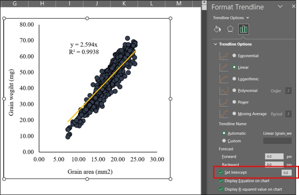
For example, when forcing the intercept to 0 using Excel, R² is calculated as 0.9938, whereas in the normal linear regression, it was 0.9219. The R² value increases when the intercept is forced to 0 because the formula for R² is simply based on R² = SSR / SST.

To address this issue, I have developed a new R package that calculates the correct R² when the intercept is forced to 0 in a simple linear regression model.

intercept0()

This R package provides the correct R² when the intercept is forced to 0 in a simple linear regression model.

This is the basic code

# install the package 
if(!require(remotes)) install.packages("remotes")
if (!requireNamespace("intercept0", quietly = TRUE)) {
  remotes::install_github("agronomy4future/intercept0")
}
library(remotes)
library(intercept0)

# model 
model= intercept0(y ~ x, data=data name)
summary(model)

---

Let’s practice the code using the actual dataset.

#to upload data
if(!require(readr)) install.packages("readr")
library(readr)
github="https://raw.githubusercontent.com/agronomy4future/raw_data_practice/main/wheat_grain_area_vs_weight.csv"
df=data.frame(read_csv(url(github),show_col_types = FALSE))

print(head(df, 5))
  grain_area grain_weight
1      15.57         43.4
2      17.14         49.7
3      16.24         45.2
4       7.85         11.0
5      14.32         36.4
.
.
.

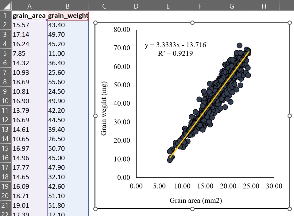
This dataset contains wheat grain area and the corresponding grain weight data. I will analyze how grain weight (y) changes in response to grain area (x).

model=lm(grain_weight ~ grain_area, data=df)
summary(model)

Call:
lm(formula = grain_weight ~ grain_area, data = df)

Residuals:
     Min       1Q   Median       3Q      Max 
-14.1497  -0.6232  -0.4314   0.8931  10.9166 

Coefficients:
            Estimate Std. Error t value Pr(>|t|)    
(Intercept) -13.7155     0.4866  -28.19   <2e-16 ***
grain_area    3.3333     0.0266  125.32   <2e-16 ***
---
Signif. codes:  0 ‘***’ 0.001 ‘**’ 0.01 ‘*’ 0.05 ‘.’ 0.1 ‘ ’ 1

Residual standard error: 2.965 on 1330 degrees of freedom
Multiple R-squared:  0.9219,	Adjusted R-squared:  0.9219 
F-statistic: 1.57e+04 on 1 and 1330 DF,  p-value: < 2.2e-16

I obtained the equation y = 3.3333x – 13.7155, where y is the grain weight (mg) and x is the grain area (mm²), with an R² value of 0.9219.

However, this model predicts negative values of y for small values of x, which is unrealistic as it implies that the grain weight would become negative when the grain area decreases beyond a certain point. To address this issue, we can simply force the intercept to be zero.

# to force intercept to 0
intercept_zero_model=lm (grain_weight ~ 0 + grain_area, data=df)
summary (intercept_zero_model)

Call:
lm(formula = grain_weight ~ 0 + grain_area, data = df)

Residuals:
     Min       1Q   Median       3Q      Max 
-13.1734  -2.5865  -0.3858   1.8437  12.9090 

Coefficients:
           Estimate Std. Error t value Pr(>|t|)    
grain_area 2.594003   0.005611   462.3   <2e-16 ***
---
Signif. codes:  0 ‘***’ 0.001 ‘**’ 0.01 ‘*’ 0.05 ‘.’ 0.1 ‘ ’ 1

Residual standard error: 3.746 on 1331 degrees of freedom
Multiple R-squared:  0.9938,	Adjusted R-squared:  0.9938 
F-statistic: 2.137e+05 on 1 and 1331 DF,  p-value: < 2.2e-16

The R² value increased when the intercept was forced to 0. If you force the intercept to 0 using Excel, you will obtain the same result.

However, this R² is incorrect, and the correct R² must be calculated to properly assess the model fit.

intercept() provides easy way to obtain the correct R²

# install the package 
if(!require(remotes)) install.packages("remotes")
if (!requireNamespace("intercept0", quietly = TRUE)) {
  remotes::install_github("agronomy4future/intercept0")
}
library(remotes)
library(intercept0)

#to upload data
if(!require(readr)) install.packages("readr")
library(readr)
github="https://raw.githubusercontent.com/agronomy4future/raw_data_practice/main/wheat_grain_area_vs_weight.csv"
df=data.frame(read_csv(url(github),show_col_types = FALSE))

print(head(df, 5))
  grain_area grain_weight
1      15.57         43.4
2      17.14         49.7
3      16.24         45.2
4       7.85         11.0
5      14.32         36.4
.
.
.

# model 
model= intercept0(grain_weight ~ grain_area, data=df)
summary(model)

Call:
lm(formula = update(formula, . ~ . - 1), data = data)

Residuals:
     Min       1Q   Median       3Q      Max 
-13.1734  -2.5865  -0.3858   1.8437  12.9090 

Coefficients:
           Estimate Std. Error t value Pr(>|t|)    
grain_area 2.594003   0.005611   462.3   <2e-16 ***
---
Signif. codes:  0 ‘***’ 0.001 ‘**’ 0.01 ‘*’ 0.05 ‘.’ 0.1 ‘ ’ 1

Residual standard error: 3.746 on 1331 degrees of freedom
Multiple R-squared:  0.9938,	Adjusted R-squared:  0.9938 
F-statistic: 2.137e+05 on 1 and 1331 DF,  p-value: < 2.2e-16

[1] Corrected R-squared: 0.8752745 

The coefficients are the same, but it provides the corrected R² in the bottom of the output. When original fitting was modified, R² should be decreased, and in this case, R² is 0.875.

Code source: agronomy4future/intercept0: This package calculates the correct R² when the intercept in a linear regression is forced to 0

---