When analyzing data, we often need to examine descriptive statistics such as standard deviation, standard error, or the coefficient of variation (CV). These are typically summarized in a short table, but in some cases, it may be necessary to include such statistics directly in the original dataset for further analysis.

Let’s upload a dataset to begin.

if(!require(readr)) install.packages("readr")
library(readr) 
github="https://raw.githubusercontent.com/agronomy4future/raw_data_practice/refs/heads/main/4_treatments_4_genotypes_with_4_blocks.csv" 
df=data.frame(read_csv(url(github), show_col_types=FALSE))

head(df,5)
  Genotype Block Treatment Yield
1      CV1     I         I  42.9
2      CV1    II         I  41.6
3      CV1   III         I  28.9
4      CV1    IV         I  30.8
5      CV2     I         I  53.3
.
.
.

I would like to calculate the mean, variance, standard deviation, standard error, 95% confidence interval, coefficient of variation, and the 25th percentile of yield data, grouped by genotype and treatment. I will use the following R code to perform these calculations.

if(!require(dplyr)) install.packages("dplyr")
library(dplyr)

summary_stats= df %>%
                  group_by(Genotype, Treatment) %>%
                     summarise(
                       n= length(Yield),
                       mean= mean(Yield, na.rm= TRUE),
                       variance= var(Yield, na.rm= TRUE),
                       sd= sd(Yield, na.rm= TRUE),
                       se= sd / sqrt(n),
                       ci_lower= mean - qt(0.975, df= n-1)*se,
                       ci_upper= mean + qt(0.975, df= n-1)*se,
                       cv= sd/mean,
                       q25= quantile(Yield, probs= 0.25, na.rm=TRUE),
                        .groups= "drop")

print(summary_stats)
   Genotype Treatment  n  mean  variance   sd    se    ci_lower ci_upper  cv      q25
 1 CV1      I          4  36.0   52.1      7.22  3.61  24.6     47.5      0.200   30.3
 2 CV1      II         4  50.6   45.3      6.73  3.37  39.9     61.3      0.133   45.7
 3 CV1      III        4  45.8   48.2      6.94  3.47  34.8     56.9      0.151   40.4
 4 CV1      IV         4  37.3   52.8      7.27  3.63  25.7     48.9      0.195   33.1
 5 CV2      I          4  50.8   212.      14.6  7.28  27.7     74.0      0.286   42.8
 6 CV2      II         4  55.4   129.      11.4  5.68  37.3     73.5      0.205   49.5
 7 CV2      III        4  53.1   134.      11.6  5.79  34.7     71.5      0.218   44.4
 8 CV2      IV         4  54.3   72.3      8.50  4.25  40.8     67.8      0.157   49.7
 9 CV3      I          4  53.9   63.7      7.98  3.99  41.2     66.6      0.148   48.9
10 CV3      II         4  51.4   69.3      8.33  4.16  38.1     64.6      0.162   46.3
11 CV3      III        4  55.9   82.1      9.06  4.53  41.5     70.3      0.162   49.2
12 CV3      IV         4  56.0   28.8      5.36  2.68  47.5     64.6      0.0957  52.5
13 CV4      I          4  61.9   114.      10.7  5.35  44.9     78.9      0.173   53.7
14 CV4      II         4  63.4   40.2      6.34  3.17  53.3     73.5      0.0999  58.3
15 CV4      III        4  57.7   124.      11.1  5.57  39.9     75.4      0.193   49.6
16 CV4      IV         4  61.2   129.      11.4  5.68  43.2     79.3      0.185   54.3

However, I would like to append these descriptive statistics to my raw dataset (df) in order to include them in my figures. To facilitate this process, I created a new R package called descriptivestat(). Below is the basic structure of the code:

data	A data frame containing the input dataset.
group_vars	Character vector of column names used to group the data
value_vars	Character vector of numeric variable names to compute statistics
output_stats	Character vector of statistics to compute. Valid options include: mean is automatically calculated and inserted to the rows v: Variance sd: Standard deviation se: Standard error ci: 95% confidence interval (LCI, UCI) cv: Coefficient of variation iqr: Interquartile range (Q1, Q2, Q3)

# upload required package
if(!require(remotes)) install.packages("remotes")
if (!requireNamespace("descriptivestat", quietly = TRUE)) {
  remotes::install_github("agronomy4future/descriptivestat", force= TRUE)
}
library(remotes)
library(descriptivestat)

I will calculate the mean, standard deviation, coefficient of variation, interquartile range, and other descriptive statistics, and append them to the original dataset.

# to calculate descriptive statistics
df1= descriptivestat(data= df, group_vars= c("Genotype", "Treatment"), 
                     value_vars= c("Yield"), 
                     output_stats= c("v","sd","se","ci","cv","iqr"))

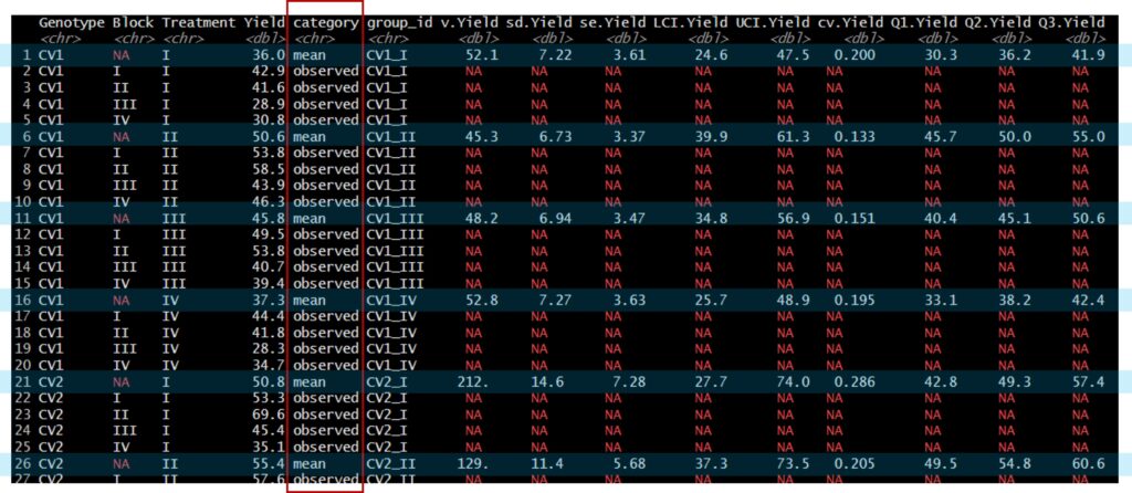
print(df1, n= Inf)

This package inserts the mean values between data rows by group, and the corresponding descriptive statistics are also added to the raw dataset.

Github: https://github.com/agronomy4future/descriptivestat

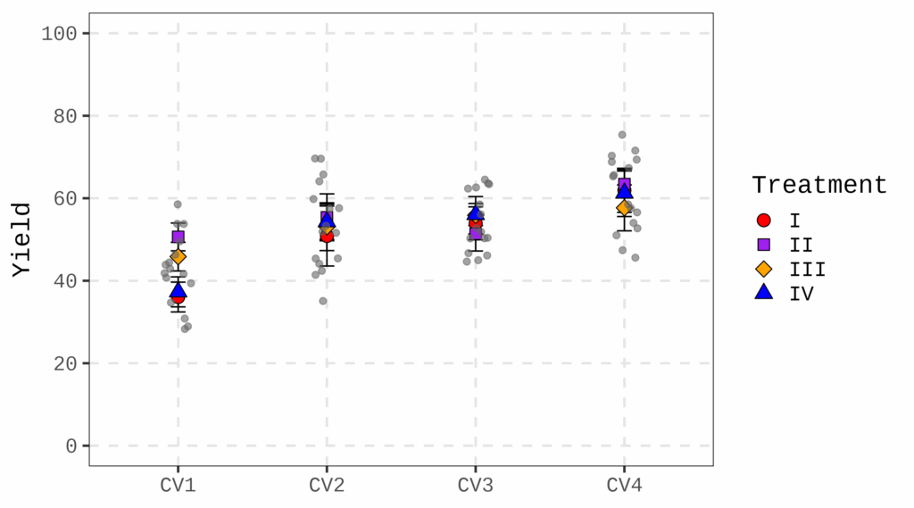
I’ll create a figure.

Fig1= ggplot() +
  geom_errorbar(data= subset(df1, category=="mean"),
                aes(x= Genotype, ymin= Yield-se.Yield, ymax=Yield+se.Yield),
                width= 0.1, color= "black") +
  
  geom_point(data= subset(df1, category=="mean"),
             aes(x= Genotype, y= Yield, fill= Treatment, shape=Treatment),
             size=4, color="black") +
  
  scale_fill_manual(name="Treatment", values= c("I"="red", "II"="purple", "III"="orange", "IV"="blue")) +
  scale_shape_manual(name="Treatment", values = c("I"=21, "II"=22, "III"=23, "IV"=24)) +
  
  geom_jitter(data= subset(df1, category=="observed"),
              aes(x= Genotype, y= Yield), width=0.1, alpha=0.6, 
              size=2, color="gray40") +
  
  scale_y_continuous(breaks=seq(0,100,20), limits = c(0,100)) +
  labs(x= NULL, y="Yield") +
  theme_classic(base_size=18, base_family="serif") +
  theme(
    legend.position="right",
    legend.key=element_rect(color="white", fill="white"),
    legend.text=element_text(family="serif", face="plain", 
                             size=15, color= "black"),
    legend.background=element_rect(fill=alpha("white", 0.5)),
    strip.background= element_rect(color= "black", fill="grey75", 
                                   linewidth= 0.5, linetype="solid"),
    panel.border= element_rect(color="black", fill=NA, linewidth=0.5),
    panel.grid.major= element_line(color="grey90", linetype="dashed"),
    axis.line= element_blank())

options(repr.plot.width=9, repr.plot.height=5)
print(Fig1)

If you would like to use standard deviation as the error bar, you can simply modify the code accordingly.

geom_errorbar(data= subset(df1, category=="mean"),
              aes(x= Genotype, ymin= Yield-sd.Yield, ymax=Yield+sd.Yield),
              width= 0.1, color= "black") +

This dataset enables visualization of both the raw data points and their means, along with standard deviation, standard error, or other descriptive statistics.

Here is another example using a large dataset.

if(!require(readr)) install.packages("readr")
library(readr) 

github="https://raw.githubusercontent.com/agronomy4future/raw_data_practice/refs/heads/main/wheat_grain_grea_and_heat_tolerance.csv" 
df=data.frame(read_csv(url(github), show_col_types=FALSE))
df = subset(df, select = -tolerance)

head(df,5)
  genotype thinning area
1      cv1  control 7.56         
2      cv1  control 7.25         
3      cv1  control 7.99         
4      cv1  control 5.86         
5      cv1  control 8.04         
.
.
.
tail(df,5)
     genotype     thinning  area 
7970      cv2 manipulation 19.71         
7971      cv2 manipulation 16.40         
7972      cv2 manipulation 21.38         
7973      cv2 manipulation 14.33         
7974      cv2 manipulation 10.83         

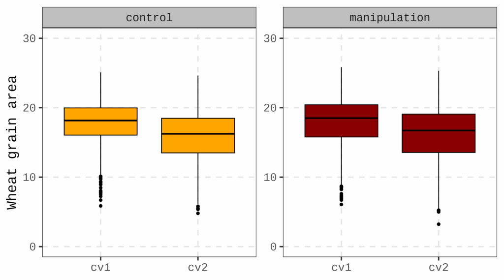
This is a large dataset used to measure wheat grain area in response to a thinning treatment applied in the field. In each plot, alternate wheat rows were removed to increase assimilate availability by reducing competition. Due to the large number of data points (7,974 datapoints), visualizing individual raw data is not practical; instead, boxplots or bar graphs would be more appropriate.

Fig2= ggplot(data=df, aes(x= genotype, y=area)) +
  geom_boxplot(aes(fill= thinning, color= thinning), color="black") +
  scale_fill_manual(name="Thinning", values= c("control"="orange", "manipulation"="darkred")) +
  scale_y_continuous(breaks=seq(0,30,10), limits= c(0,30)) +
  facet_wrap(~ thinning, scales= "free") +
  labs(x= NULL, y="Wheat grain area") +
  theme_classic(base_size=18, base_family="serif") +
  theme(
    legend.position="none",
    legend.key=element_rect(color="white", fill="white"),
    legend.text=element_text(family="serif", face="plain",
                             size=15, color= "black"),
    legend.background=element_rect(fill=alpha("white", 0.5)),
    strip.background= element_rect(color= "black", fill="grey75",
                      linewidth= 0.5, linetype="solid"),
    panel.border= element_rect(color="black", fill=NA, linewidth=0.5),
    panel.grid.major= element_line(color="grey90", linetype="dashed"),
    axis.line= element_blank())

options(repr.plot.width=9, repr.plot.height=5)
print(Fig2)

However, I would like to visualize both the raw data and its variability. In this case, the descriptivestat() package is useful for that purpose.

First, I will output the standard deviation and interquartile range (IQR) for this dataset.

df1= descriptivestat(data= df, group_vars= c("genotype", "thinning"), 
                     value_vars= c("area"), 
                     output_stats= c("sd","iqr"))

print(head(df1, 5))
  genotype thinning area  category  group_id     sd.area Q1.area Q2.area Q3.area
1 cv1      control  17.8  mean      cv1_control  2.97    16.1    18.2    20.0
2 cv1      control  7.56  observed  cv1_control  NA       NA      NA      NA  
3 cv1      control  7.25  observed  cv1_control  NA       NA      NA      NA  
4 cv1      control  7.99  observed  cv1_control  NA       NA      NA      NA  
5 cv1      control  5.86  observed  cv1_control  NA       NA      NA      NA  
.
.
.   

This graph will help illustrate both individual variability and the overall trend in the data.

Fig3= ggplot() +
  geom_jitter(data= subset(df1, category=="observed"),
              aes(x= genotype, y= area), width=0.2, alpha=0.7,
              size=2, color="gray75") +

  geom_errorbar(data= subset(df1, category=="mean"),
                aes(x= genotype, ymin= area-sd.area, ymax=area+sd.area),
                width= 0.1, color= "black") +

  geom_point(data= subset(df1, category=="mean"),
             aes(x= genotype, y= area, fill= thinning, shape=thinning),
             size=4, color="black") +

  scale_fill_manual(name="Thinning", values= c("control"="orange", "manipulation"="red")) +
  scale_shape_manual(name="Thinning", values = c("control"=21, "manipulation"=22)) +            
  scale_y_continuous(breaks=seq(0,30,10), limits = c(0,30)) +
  facet_wrap(~ thinning, scales = "free") +
  labs(x= NULL, y="Wheat grain area") +
  theme_classic(base_size=18, base_family="serif") +
  theme(
    legend.position="none",
    legend.key=element_rect(color="white", fill="white"),
    legend.text=element_text(family="serif", face="plain",
                             size=15, color= "black"),
    legend.background=element_rect(fill=alpha("white", 0.5)),
    strip.background= element_rect(color= "black", fill="grey75",
                      linewidth= 0.5, linetype="solid"),
    panel.border= element_rect(color="black", fill=NA, linewidth=0.5),
    panel.grid.major= element_line(color="grey90", linetype="dashed"),
    axis.line= element_blank()
  )

options(repr.plot.width=9, repr.plot.height=5)
print(Fig3)

Since the descriptivestat() package appends the mean and other descriptive statistics to the raw dataset, we can easily use them for visualization.

If you want to use upper and lower percentiles as error bars, you can simply modify the code as shown below.

  geom_errorbar(data= subset(df1, category=="mean"),
                aes(x= genotype, ymin= area-(area-Q1.area), ymax=area+(Q3.area-area)),
                width= 0.1, color= "black") +

When compared to a boxplot, the upper and lower percentiles are exactly the same as those represented by the box boundaries.

Which type of graph do you prefer? While a boxplot effectively summarizes data variability using quartiles, the graph generated with the descriptivestat() package provides a clearer visualization by displaying the actual raw data alongside the mean and other descriptive statistics.

full code: r_code/Embedding_Key_Descriptive_Statistics_within_Original_Data_(Feat__descriptivestat).ipynb at main · agronomy4future/r_code

---