Understanding Multiple Linear Regression Easily (Part 2: Calculating the Coefficient of Determination Manually)

□ Understanding Multiple Linear Regression Easily (Part 1: Calculating the Regression Equation Manually)

In the previous post, we explained how to manually calculate the regression equation in multiple linear regression analysis. Now, in this post, I will explain how to calculate the coefficient of determination (R²) in multiple linear regression analysis.

No.	Yield (y_i)	Time (x_i1)	Moisture (x_i2)
1	4.3	4	0.2
2	5.5	5	0.2
3	6.8	6	0.2
4	8.0	7	0.2
5	4.0	4	0.3
6	5.2	5	0.3
7	6.6	6	0.3
8	7.5	7	0.3
9	2.0	4	0.4
10	4.0	5	0.4
11	5.7	6	0.4
12	6.5	7	0.4

To calculate the coefficient of determination (R²), we need to compute simple linear regression equations for each independent variable (x). When analyzing the linear regression equations for Time and Moisture respectively, you can obtain the following results:

<strong>### Yield in response to time</strong>
model= lm (yield ~ time, data=dataA)
summary(model)

Coefficients:
            Estimate Std. Error t value Pr(>|t|)    
(Intercept)  -1.7333     1.1652  -1.488    0.168    
time          1.3167     0.2076   6.342 8.44e-05 ***

<strong>### Yield in response to moisture</strong>
model= lm (yield ~ moisture, data=dataA)
summary(model)

Coefficients:
            Estimate Std. Error t value Pr(>|t|)   
(Intercept)    7.908      1.818   4.350  0.00144 **
moisture      -8.000      5.847  -1.368  0.20119   

Therefore, 
Time: ŷ<sub>i</sub>=-1.73 + 1.31 x<sub>i1</sub>
Moisture: ŷ<sub>i</sub>=7.9 - 8.0* x<sub>i2</sub>

Next, I will use each of these regression equations to partition the data.

1) Time

No.	Yield (y_i)	Time (x_i1)	Time: `ŷ_i=-1.73+1.31x_i1`	Data: `(y_i - ȳ)²`	Fit: `(ŷ_i - ȳ)²`	Error: `(ŷ_i - y_i)²`
1	4.3	4	3.53	1.5	3.9	0.6
2	5.5	5	4.85	0.0	0.4	0.4
3	6.8	6	6.17	1.7	0.4	0.4
4	8.0	7	7.48	6.2	3.9	0.3
5	4.0	4	3.53	2.3	3.9	0.2
6	5.2	5	4.85	0.1	0.4	0.1
7	6.6	6	6.17	1.2	0.4	0.2
8	7.5	7	7.48	4.0	3.9	0.0
9	2.0	4	3.53	12.3	3.9	2.4
10	4.0	5	4.85	2.3	0.4	0.7
11	5.7	6	6.17	0.0	0.4	0.2
12	6.5	7	7.48	1.0	3.9	1.0
Mean	ȳ= 5.5			SST: `Σ(y_i - ȳ)²` 32.5	SSR: `Σ(ŷ_i - ȳ)²` 26.0	SSE: `Σ(ŷ_i - y_i)²` 6.5

2) Moisture

No.	Yield (y_i)	Moisture (x_i1)	Moisture: `ŷ_i=7.9-8.0*x_i2`	Data: `(y_i - ȳ)²`	Fit: `(ŷ_i - ȳ)²`	Error: `(ŷ_i - y_i)²`
1	4.3	0.2	6.31	1.5	0.6	4.0
2	5.5	0.2	6.31	0.0	0.6	0.7
3	6.8	0.2	6.31	1.7	0.6	0.2
4	8.0	0.2	6.31	6.2	0.6	2.9
5	4.0	0.3	5.51	2.3	0.0	2.3
6	5.2	0.3	5.51	0.1	0.0	0.1
7	6.6	0.3	5.51	1.2	0.0	1.2
8	7.5	0.3	5.51	4.0	0.0	4.0
9	2.0	0.4	4.71	12.3	0.6	7.3
10	4.0	0.4	4.71	2.3	0.6	0.5
11	5.7	0.4	4.71	0.0	0.6	1.0
12	6.5	0.4	4.71	1.0	0.6	3.2
Mean	ȳ= 5.5			SST: `Σ(y_i - ȳ)²` 32.5	SSR: `Σ(ŷ_i - ȳ)²` 5.1	SSE: `Σ(ŷ_i - y_i)²` 27.3

Now, let’s create an ANOVA table.

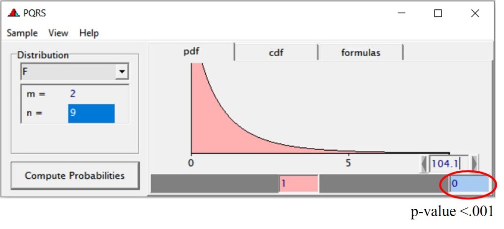
Source	df	SS	MS	F	p-value
Model	2	SSR: 26.0 +5.1 = 31.1	31.1 / 2 =15.6	15.6 / 0.1 = 104.1	<.001
Error	9	SSE: 32.5 – 31.1 = 1.3	1.3 / 9 = 0.1
Total	11	SST: 32.5	32.5 / 11 = 2.95

Then, the coefficient of determination (R^2) is calculated using the following formula:

31.1 / 32.5 ≈ 0.96