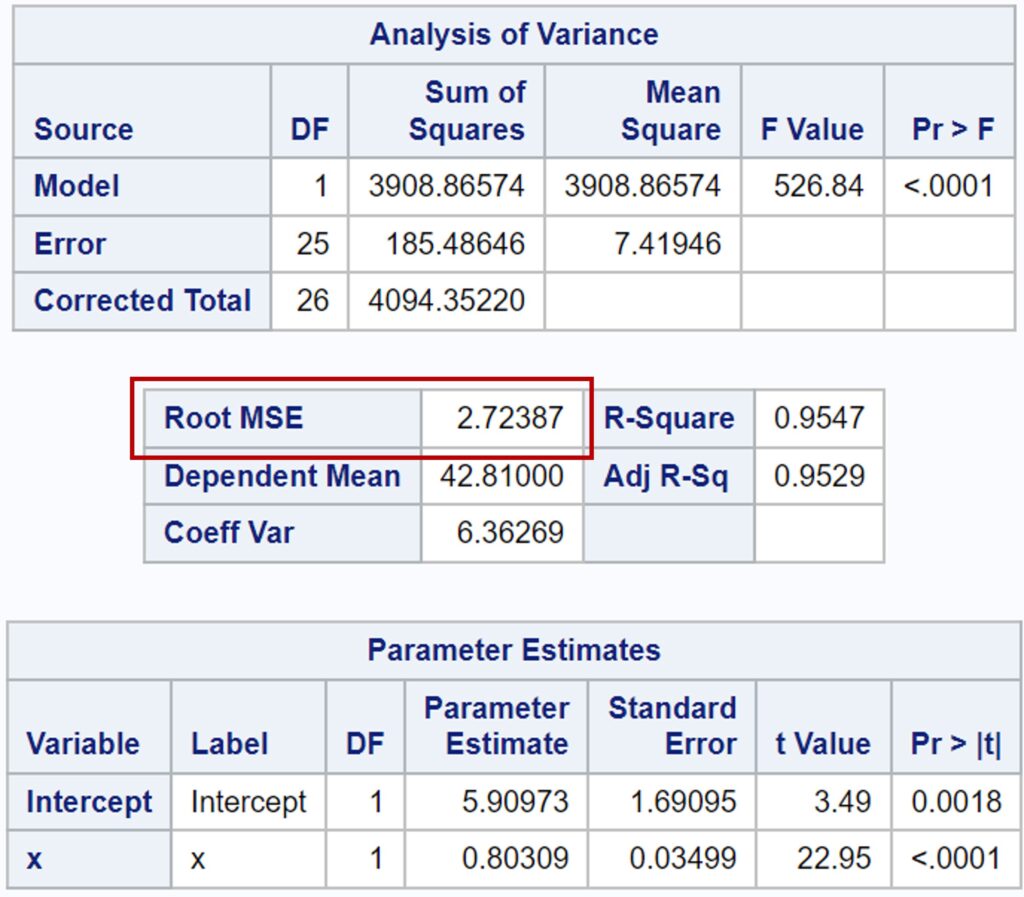
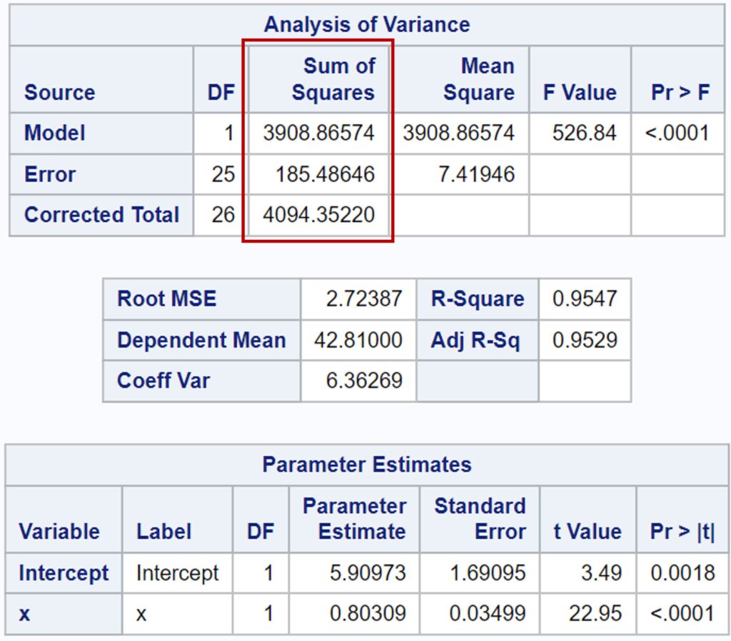
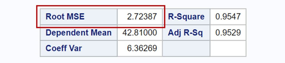
---

When running statistical programs, you might encounter RMSE (Root Mean Square Error). For example, the table below shows RMSE values obtained from SAS, indicating that it is ca. 2.72.

I’m curious about how RMSE is calculated. Below is the equation for RMSE.

First, calculate the difference between the estimated and observed values: (ŷi - yi), and then square the difference: (ŷi - yi)².
 
Second, calculate the sum of squares: Σ(ŷi - yi)². 

Third, divide the sum of squares by the number of samples (n): Σ(ŷi - yi)²/n. 

Finally, take the square root of the result: √(Σ(ŷi - yi)²/n).

The calculation of the sum of squares, Σ(ŷi - yi)², is a similar concept to the sum of squared errors (SSE). When SSE is divided by the degrees of freedom, it becomes the mean squared error (MSE). Therefore, we can deduce that RMSE is the square root of MSE: RMSE = √MSE.

In SAS, MSE is 7.41946. Thus, I calculated the RMSE as √7.41946 ≈ 2.72, which is the same value that SAS provided. Therefore, we can easily calculate the RMSE as √MSE.

However, one question remains: How do we calculate MSE? While statistical programs automatically calculate it, understanding how MSE is calculated is essential to fully comprehend our data.

How to calculate MSE in simple linear regression?

[Step 1] Regression analysis

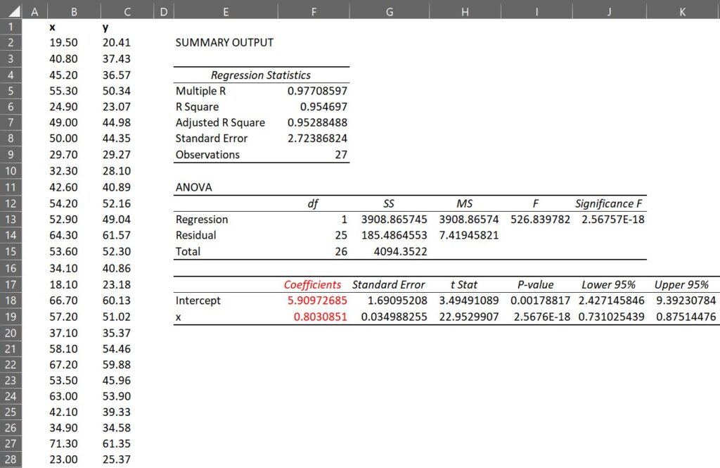
Here is one data (You can copy and paste the data below into Excel).

x	y
19.50	20.41
40.80	37.43
45.20	36.57
55.30	50.34
24.90	23.07
49.00	44.98
50.00	44.35
29.70	29.27
32.30	28.10
42.60	40.89
54.20	52.16
52.90	49.04
64.30	61.57
53.60	52.30
34.10	40.86
18.10	23.18
66.70	60.13
57.20	51.02
37.10	35.37
58.10	54.46
67.20	59.88
53.50	45.96
63.00	53.90
42.10	39.33
34.90	34.58
71.30	61.35
23.00	25.37

By performing a regression analysis on the dataset in Excel, you can obtain an equation that relates the dependent variable (y) to the independent variable (x): ŷ = 5.90 + 80309x. This equation can be used to predict y for any given value of x within the range of the dataset.

In R, the code would be like below.

x=c(19.5,40.8,45.2,55.3,24.9,49,50,29.7,32.3,42.6,54.2,52.9,64.3,53.6,34.1,18.1,66.7,57.2,37.1,58.1,67.2,53.5,63,42.1,34.9,71.3,23)
y=c(20.41,37.43,36.57,50.34,23.07,44.98,44.35,29.27,28.10,40.89,52.16,49.04,61.57,52.3,40.86,23.18,60.13,51.02,35.37,54.46,59.88,45.96,53.9,39.33,34.58,61.35,25.37)
dataA=data.frame (x,y)

#Linear regression
summary (lm (y ~ x, data=dataA))
Coefficients:
            Estimate Std. Error t value Pr(>|t|)    
(Intercept)  5.90973    1.69095   3.495  0.00179 ** 
x            0.80309    0.03499  22.953  < 2e-16 ***
---
Signif. codes:  0 ‘***’ 0.001 ‘**’ 0.01 ‘*’ 0.05 ‘.’ 0.1 ‘ ’ 1

[Step 2] Calculate estimated ŷ

As we have obtained ŷ = 5.90 + 0.80309x, we can calculate the estimated value (ŷ). For example, if we take x to be 19.50, the estimated value ŷ will be 21.57, which can be calculated as 5.90 + 0.80309 * 19.50.

x	y	ŷ
19.50	20.41	21.57
40.80	37.43	38.68
45.20	36.57	42.21
55.30	50.34	50.32
24.90	23.07	25.91
49.00	44.98	45.26
50.00	44.35	46.06
29.70	29.27	29.76
32.30	28.10	31.85
42.60	40.89	40.12
54.20	52.16	49.44
52.90	49.04	48.39
64.30	61.57	57.55
53.60	52.30	48.96
34.10	40.86	33.30
18.10	23.18	20.45
66.70	60.13	59.48
57.20	51.02	51.85
37.10	35.37	35.70
58.10	54.46	52.57
67.20	59.88	59.88
53.50	45.96	48.88
63.00	53.90	56.50
42.10	39.33	37.72
34.90	34.58	33.94
71.30	61.35	63.17
23.00	25.37	24.38

In R, the code would be like below.

dataA$yi= 5.90973 + 0.80309*dataA$x

head(dataA,5)
x	y	yi
19.5	20.41	21.56998
40.8	37.43	38.67580
45.2	36.57	42.20940
55.3	50.34	50.32061
24.9	23.07	25.90667
.
.
.

[Step 3] Calculate each sum of squares

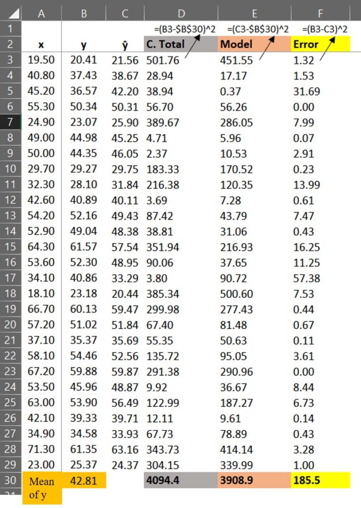
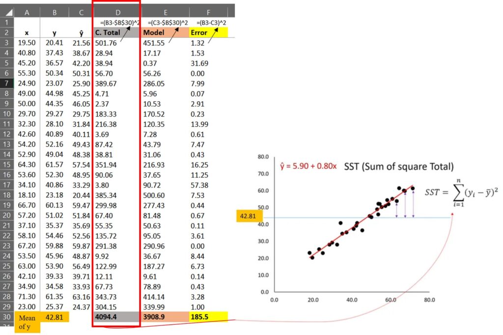
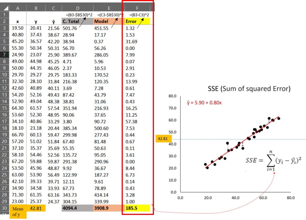
First, let’s do data partitioning.

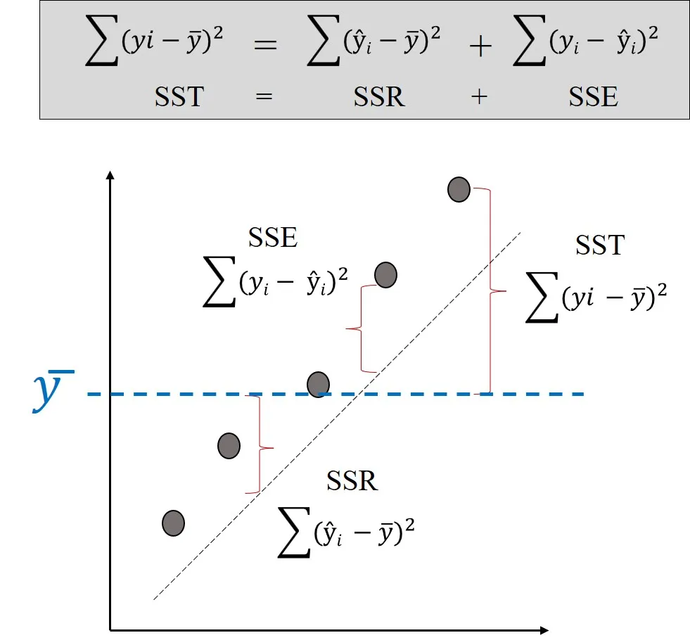
This partitioning is based on the below concept.

Recommended article
□ Simple linear regression (5/5)- R_squared

The sum of squares values calculated by Excel match those provided by SAS.

In R, we can also conduct data partitioning.

dataA$SST= round((dataA$y - mean(dataA$y))^2,digit=2)
dataA$SSR= round((dataA$yi - mean(dataA$y))^2,digit=2)
dataA$SSE= round((dataA$y - dataA$yi)^2,digit=2)

head(dataA,5)
x	y	yi	   SST	    SSR	      SSE
19.5	20.41	21.56998   501.76   451.14    1.35
40.8	37.43	38.67580   28.94    17.09     1.55
45.2	36.57	42.20940   38.94    0.36      31.80
55.3	50.34	50.32061   56.70    56.41     0.00
24.9	23.07	25.90667   389.67   285.72    8.05
.
.
.

SST=sum(dataA$SST)  ≈ 4094.4
SSR=sum(dataA$SSR)  ≈ 3908.9
SSE=sum(dataA$SSE)  ≈ 185.5

[Step 4] Calculate Mean squared Error (MSE)

The sum of squares total (SST) can be partitioned into the sum of squares due to regression (SSR) and the sum of squares of errors (SSE).

SST (Total)= SSR (Model) + SSE (Error)

That is, 4094.4= 3908.9 + 185.5

The table below shows the sources of variance for regression.

Source	Degrees of Freedom	Sum of Squares	Mean Square	F-ratio	p-value
Model	p	SSR	MSR = SSR/p	MSR/MSE	p-value
Error	n-p-1	SSE	MSE = SSE/(n-p-1)
Total	n-1	SST

---

As we have already calculated SST, SSR, and SSE, we can easily compute their mean squared values by dividing each of them by the number of samples (n), which is 27 in our case. Based on this, we can construct the ANOVA table, which would look something like this.

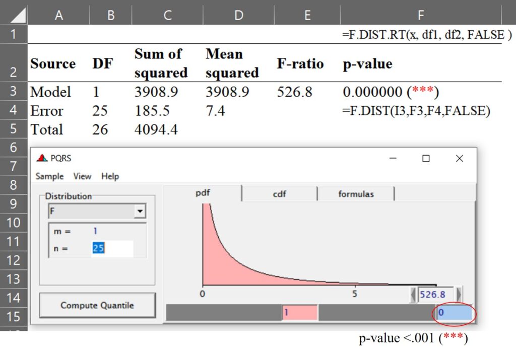
MSE was calculated as 7.4 (=185.5 / (27 – 2)). It’s the same value as what SAS provided.

In R, we can obtain MSE using below code.

anova (lm (y ~ x, data=dataA))
           Df	Sum Sq	   Mean Sq	F value	    Pr(>F)
x	   1	3908.8657  3908.865745	526.8398    2.567573e-18
Residuals  25	185.4865   7.419458	

Then, RMSE will be √7.4 ≈ 2.72. It’s the same value as what SAS provide.

Wrap up!!

1) How to calculate sum of squares total (SST)?

(20.41 – 42.81)2 + (37.43 – 42.81)2 + … + (25.37 – 42.81)2 = 4094.4

First, we calculated the difference between each observed value (black dot in the below graph) and the mean of the observed values (blue line in the below graph), and calculated the sum of squares of each difference; Σ(yi - ȳ)2.

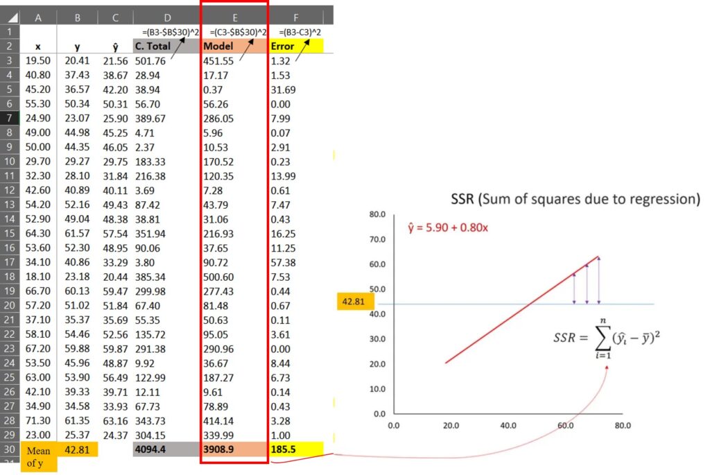
2) How to calculate Model (SSR)?

(21.56 – 42.81)2 + (38.67 – 42.81)2 + … + (24.37 – 42.81)2 = 3908.9

First, we calculated the difference between each estimated value (red line in the below graph) and the mean of the observed values (blue line in the below graph), and calculated the sum of squares of each difference; Σ(ŷi - ȳ)2.

3) How to calculate SSE?

(21.56 – 20.41)2 + (38.67 – 37.43)2 + … + (24.37 – 25.37)2 = 185.5

First, we calculated the difference between each estimated value (red line in the below graph) and each observed value (black dot in the below graph), and calculated the sum of squares of each difference; Σ(ŷi - yi)2.

That’s why SST = SSR + SSE

Eventually, MSE (also called Residuals) explains how far data points are dispersed from the regression line, and RMSE (=√MSE) is explained as the standard deviation (we put √ in variance) of the residuals.

How about calculating the differences between two variables without fitting?

Sometimes, I see many people obtain RMSE, simply calculating the differences between two variables like below.

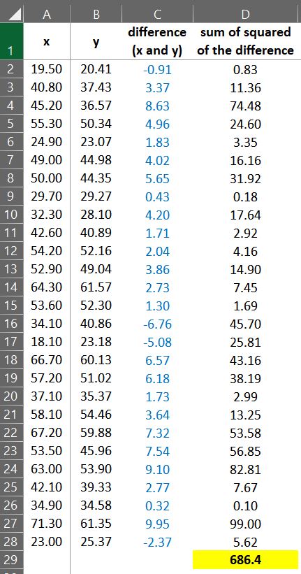
They squared each difference(xi - yi)2, and calculated the sum of squares; Σ(xi - yi)2, and then divided by number of samples (n); Σ(xi - yi)2 / n

i.e. 684.4 / 27 ≈ 25.35.

They say it would be MSE and RMSE will be √25.35 ≈ 5.04

In R, the calculation would be like below.

dataA$Difference= dataA$x- dataA$y
dataA$Difference_square= (dataA$x- dataA$y)^2

head(dataA,5)
x	y	yi	  SST	  SSR	  SSE	 Difference   Difference_square
19.5	20.41	21.56998  501.76  451.14  1.35	 -0.91	      0.8281
40.8	37.43	38.67580  28.94	  17.09	  1.55	 3.37	      11.3569
45.2	36.57	42.20940  38.94	  0.36	  31.80	 8.63	      74.4769
55.3	50.34	50.32061  56.70	  56.41	  0.00	 4.96	      24.6016
24.9	23.07	25.90667  389.67  285.72  8.05	 1.83	      3.3489
.
.
.

sqrt(sum(dataA$Difference_square)/length(dataA$y))
# 5.042012

Then RMSE will be ≈ 5.04

This value is different from what we calculated, 2.72. This would be an issue about how to interpret RMSE.

This raises an issue about how to interpret RMSE, but in order to understand this, we first need to understand the difference from √Σ(ŷi - yi)2/(n-2) to Σ(xi - yi)2/n.

The reason why I point out this issue is people simply believe what the statistical software provides. For example, R provides a simple code to calculate RMSE.

if(!require(Metrics)) install.packages("Metrics")
library(Metrics)

rmse= rmse(dataA$x, dataA$y)

print(rmse)
5.042012

Now it’s 5.04. This is about Σ(xi - yi)2/n, not √Σ(ŷi - yi)2/(n-2). If you just accept this RMSE value without any doubts, you never explain why this value is different from 2.72 which is calculated as √Σ(ŷi - yi)2/(n-2)

Many people tend to overlook this issue, assuming that there must be an error in the calculation. However, it is important to note that the discrepancy is not due to an error, but rather a difference in the calculation methods. It is important to not simply rely on the output provided by statistical programs, but rather to take the time to understand the underlying principles and calculations that are used. By doing so, we can gain a deeper understanding of our data and feel more confident in your results.

---

---

Your donation will help us create high-quality content.
PayPal @agronomy4furure / Venmo @agronomy4furure / Zelle @agronomy4furure